The calculation of a beam for bending "manually", in an old-fashioned way, allows you to learn one of the most important, beautiful, clearly mathematically verified algorithms of the science of the strength of materials. The use of numerous programs such as "entered the initial data ...
...– get an answer” allows the modern engineer today to work much faster than his predecessors a hundred, fifty and even twenty years ago. However, with such a modern approach, the engineer is forced to fully trust the authors of the program and eventually ceases to "feel the physical meaning" of the calculations. But the authors of the program are people, and people make mistakes. If this were not so, then there would not be numerous patches, releases, "patches" for almost any software. Therefore, it seems to me that any engineer should sometimes be able to "manually" check the results of calculations.
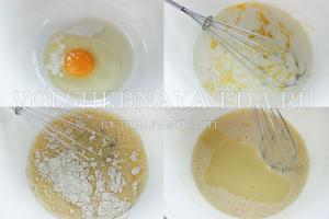
Help (cheat sheet, memo) for calculating beams for bending is shown below in the figure.
 Let's use a simple everyday example to try to use it. Let's say I decided to make a horizontal bar in the apartment. A place has been determined - a corridor one meter twenty centimeters wide. On opposite walls at the required height opposite each other, I securely fasten the brackets to which the beam-beam will be attached - a bar of St3 steel with an outer diameter of thirty-two millimeters. Will this beam support my weight plus additional dynamic loads that will arise during exercise?
We draw a diagram for calculating the beam for bending. Obviously, the application scheme will be the most dangerous. external load, when I start to pull myself up, clinging with one hand to the middle of the crossbar.
 Initial data:
F1 \u003d 900 n - the force acting on the beam (my weight) without taking into account the dynamics
d \u003d 32 mm - the outer diameter of the bar from which the beam is made
E = 206000 n/mm^2 is the modulus of elasticity of the St3 steel beam material
[σi] = 250 n/mm^2 - allowable bending stresses (yield strength) for the material of the St3 steel beam
Border conditions:
Мx (0) = 0 n*m – moment at point z = 0 m (first support)
Мx (1.2) = 0 n*m – moment at point z = 1.2 m (second support)
V (0) = 0 mm - deflection at point z = 0 m (first support)
V (1.2) = 0 mm - deflection at point z = 1.2 m (second support)
Calculation:
1. First, we calculate the moment of inertia Ix and the moment of resistance Wx of the beam section. They will be useful to us in further calculations. For a circular section (which is the section of the bar):
Ix = (π*d^4)/64 = (3.14*(32/10)^4)/64 = 5.147 cm^4
Wx = (π*d^3)/32 = ((3.14*(32/10)^3)/32) = 3.217 cm^3
2. We compose equilibrium equations for calculating the reactions of the supports R1 and R2:
Qy = -R1+F1-R2 = 0
Mx (0) = F1*(0-b2) -R2*(0-b3) = 0
From the second equation: R2 = F1*b2/b3 = 900*0.6/1.2 = 450 n
From the first equation: R1 = F1-R2 = 900-450 = 450 n
3. Let's find the angle of rotation of the beam in the first support at z = 0 from the deflection equation for the second section:
V (1.2) = V (0)+U (0)*1.2+(-R1*((1.2-b1)^3)/6+F1*((1.2-b2)^3)/6)/
U (0) = (R1*((1.2-b1)^3)/6 -F1*((1.2-b2)^3)/6)/(E*Ix)/1,2 =
= (450*((1.2-0)^3)/6 -900*((1.2-0.6)^3)/6)/
/(206000*5.147/100)/1.2 = 0.00764 rad = 0.44˚
4.
We compose equations for constructing diagrams for the first section (0 Shear force: Qy (z) = -R1 Bending moment: Mx (z) = -R1*(z-b1) Rotation angle: Ux (z) = U (0)+(-R1*((z-b1)^2)/2)/(E*Ix) Deflection: Vy (z) = V (0)+U (0)*z+(-R1*((z-b1)^3)/6)/(E*Ix) z = 0 m: Qy (0) = -R1 = -450 n Ux(0) = U(0) = 0.00764 rad Vy(0)=V(0)=0mm z = 0.6 m: Qy (0.6) = -R1 = -450 n Mx (0.6) \u003d -R1 * (0.6-b1) \u003d -450 * (0.6-0) \u003d -270 n * m Ux (0.6) = U (0)+(-R1*((0.6-b1)^2)/2)/(E*Ix) = 0.00764+(-450*((0.6-0)^2)/2)/(206000*5.147/100) = 0 rad Vy (0.6) = V (0)+U (0)*0.6+(-R1*((0.6-b1)^3)/6)/(E*Ix) = 0+0.00764*0.6+(-450*((0.6-0)^3)/6)/ (206000*5.147/100) = 0.003 m The beam will sag in the center by 3 mm under the weight of my body. I think this is an acceptable deflection. 5.
We write the diagram equations for the second section (b2 Shear force: Qy (z) = -R1+F1 Bending moment: Mx (z) = -R1*(z-b1)+F1*(z-b2) Rotation angle: Ux (z) = U (0)+(-R1*((z-b1)^2)/2+F1*((z-b2)^2)/2)/(E*Ix) Deflection: Vy (z) = V (0)+U (0)*z+(-R1*((z-b1)^3)/6+F1*((z-b2)^3)/6)/( E*Ix) z = 1.2 m: Qy (1,2) = -R1+F1 = -450+900 = 450 n Мx (1,2) = 0 n*m Ux (1,2) = U (0)+(-R1*((1,2-b1)^2)/2+F1*((1,2-b2)^2)/2)/(E* ix) = 0,00764+(-450*((1,2-0)^2)/2+900*((1,2-0,6)^2)/2)/ /(206000*5.147/100) = -0.00764 rad Vy (1.2) = V (1.2) = 0 m 6.
We build diagrams using the data obtained above. 7.
We calculate the bending stresses in the most loaded section - in the middle of the beam and compare with the allowable stresses: σi \u003d Mx max / Wx \u003d (270 * 1000) / (3.217 * 1000) \u003d 84 n / mm ^ 2 σi = 84 n/mm^2< [σи] = 250 н/мм^2 In terms of bending strength, the calculation showed a threefold margin of safety - the horizontal bar can be safely made from an existing bar with a diameter of thirty-two millimeters and a length of one thousand two hundred millimeters. Thus, you can now easily calculate the beam for bending "manually" and compare with the results obtained in the calculation using any of the numerous programs presented on the Web. I ask those who RESPECT the work of the author to SUBSCRIBE to the announcements of articles.
86 comments on "Calculation of a beam for bending - "manually"!" Building a diagram Q.
Let's build a plot M
method characteristic points. We arrange points on the beam - these are the points of the beginning and end of the beam ( D,A
), concentrated moment ( B
), and also note as a characteristic point the middle of a uniformly distributed load ( K
) is an additional point for constructing a parabolic curve. Determine bending moments at points. Rule of signs cm. - . The moment in IN
will be defined as follows. First let's define: point TO
let's take in middle area with a uniformly distributed load. Building a diagram M
. Plot AB
– parabolic curve(rule of "umbrella"), plot BD
– straight oblique line. For a beam, determine the support reactions and plot bending moment diagrams ( M) and shear forces ( Q).
Compiling equilibrium equations. Examination Write down the values R A
And R B
on calculation scheme. 2. Plotting transverse forces method sections. We place the sections on characteristic areas(between changes). According to the dimensional thread - 4 sections, 4 sections. sec. 1-1 move left. The section passes through the section with uniformly distributed load, note the size z 1
to the left of the section before the beginning of the section. Plot length 2 m. Rule of signs For Q
- cm. We build on the found value diagramQ.
sec. 2-2 move right. The section again passes through the area with a uniformly distributed load, note the size z 2
to the right of the section to the beginning of the section. Plot length 6 m. Building a diagram Q.
sec. 3-3 move right. sec. 4-4 move to the right. We are building diagramQ.
3. Construction diagrams M method characteristic points. characteristic point- a point, any noticeable on the beam. These are the dots A, IN, WITH, D
, as well as the point TO
, wherein Q=0
And bending moment has an extremum. also in middle console put an additional point E, since in this area under a uniformly distributed load the diagram M described crooked line, and it is built, at least, according to 3
points. So, the points are placed, we proceed to determine the values in them bending moments. Rule of signs - see.. Plots NA, AD
– parabolic curve(the “umbrella” rule for mechanical specialties or the “sail rule” for construction), sections DC, SW
– straight slanted lines. Moment at a point D
should be determined both left and right from the point D
. The very moment in these expressions Excluded. At the point D
we get two values from difference by the amount m
– jump to its size. Now we need to determine the moment at the point TO
(Q=0). However, first we define point position TO
, denoting the distance from it to the beginning of the section by the unknown X
. T. TO
belongs second characteristic area, shear force equation(see above) But the transverse force in t. TO
is equal to 0
, A z 2
equals unknown X
. We get the equation: Now knowing X,
determine the moment at a point TO
on the right side. Building a diagram M
. The construction is feasible for mechanical specialties, postponing positive values up from the zero line and using the "umbrella" rule. For a given scheme of a cantilever beam, it is required to plot the diagrams of the transverse force Q and the bending moment M, perform a design calculation by selecting a circular section. Material - wood, design resistance of the material R=10MPa, M=14kN m, q=8kN/m There are two ways to build diagrams in a cantilevered beam with rigid embedding - the usual one, having previously determined the support reactions, and without defining the support reactions, if we consider the sections, going from the free end of the beam and discarding the left side with the embedding. Let's build diagrams ordinary way. 1. Define support reactions. Uniformly distributed load q replace the conditional force Q= q 0.84=6.72 kN In a rigid embedment, there are three support reactions - vertical, horizontal and moment, in our case, the horizontal reaction is 0. Let's find vertical support reaction R A And reference moment M A from the equilibrium equations. In the first two sections on the right, there is no transverse force. At the beginning of a section with a uniformly distributed load (right) Q=0, in the back - the magnitude of the reaction R.A. We solve equation (1), reduce by EI Static Indeterminacy Revealed, the value of the "extra" reaction is found. You can start plotting Q and M diagrams for a statically indeterminate beam... We sketch the given beam scheme and indicate the reaction value Rb. In this beam, the reactions in the termination can not be determined if you go to the right. Building plots Q for a statically indeterminate beam Plot Q. Plotting M We define M at the point of extremum - at the point TO. First, let's define its position. We denote the distance to it as unknown " X". Then We plot M. Determination of shear stresses in an I-section. Consider the section I-beam. S x \u003d 96.9 cm 3; Yx=2030 cm 4; Q=200 kN To determine the shear stress, it is used formula Compute maximum shear stress: Let us calculate the static moment for top shelf: Now let's calculate shear stresses: We are building shear stress diagram: Design and verification calculations. For a beam with constructed diagrams of internal forces, select a section in the form of two channels from the condition of strength for normal stresses. Check the strength of the beam using the shear strength condition and the energy strength criterion. Given: Let's show a beam with constructed plots Q and M According to the diagram of bending moments, the dangerous is section C, in which M C \u003d M max \u003d 48.3 kNm. Strength condition for normal stresses for this beam has the form σ max \u003d M C / W X ≤σ adm . It is necessary to select a section from two channels. For a section in the form of two channels, according to accept two channels №20a, the moment of inertia of each channel I x =1670cm 4, Then axial moment of resistance of the entire section: Overvoltage (undervoltage) at dangerous points, we calculate according to the formula: Then we get undervoltage: Now let's check the strength of the beam, based on strength conditions for shear stresses. According to diagram of shear forces dangerous are sections in section BC and section D. As can be seen from the diagram, Q max \u003d 48.9 kN. Strength condition for shear stresses looks like: For channel No. 20 a: static moment of the area S x 1 \u003d 95.9 cm 3, moment of inertia of the section I x 1 \u003d 1670 cm 4, wall thickness d 1 \u003d 5.2 mm, average shelf thickness t 1 \u003d 9.7 mm , channel height h 1 \u003d 20 cm, shelf width b 1 \u003d 8 cm. For transverse sections of two channels: S x \u003d 2S x 1 \u003d 2 95.9 \u003d 191.8 cm 3, I x \u003d 2I x 1 \u003d 2 1670 \u003d 3340 cm 4, b \u003d 2d 1 \u003d 2 0.52 \u003d 1.04 cm. Determining the value maximum shear stress: τ max \u003d 48.9 10 3 191.8 10 -6 / 3340 10 -8 1.04 10 -2 \u003d 27 MPa. As seen, τ max<τ adm
(27MPa<75МПа). Hence, strength condition is met. We check the strength of the beam according to the energy criterion. Out of consideration diagrams Q and M follows that section C is dangerous, in which M C =M max =48.3 kNm and Q C =Q max =48.9 kN. Let's spend analysis of the stress state at the points of section C Let's define normal and shear stresses at several levels (marked on the section diagram) Level 1-1: y 1-1 =h 1 /2=20/2=10cm. Normal and tangent voltage: Main voltage: Level 2-2: y 2-2 \u003d h 1 / 2-t 1 \u003d 20 / 2-0.97 \u003d 9.03 cm. Main stresses: Level 3-3: y 3-3 \u003d h 1 / 2-t 1 \u003d 20 / 2-0.97 \u003d 9.03 cm. Normal and shear stresses: Main stresses: Extreme shear stresses: Level 4-4: y 4-4 =0. (in the middle, the normal stresses are equal to zero, the tangential stresses are maximum, they were found in the strength test for tangential stresses) Main stresses: Extreme shear stresses: Level 5-5: Normal and shear stresses: Main stresses: Extreme shear stresses: Level 6-6: Normal and shear stresses: Main stresses: Extreme shear stresses: Level 7-7: Normal and shear stresses: Main stresses: Extreme shear stresses: According to the performed calculations stress diagrams σ, τ, σ 1 , σ 3 , τ max and τ min are presented in fig. Analysis these diagram shows, which is in the cross section of the beam dangerous points are at level 3-3 (or 5-5), in which: Using energy criterion of strength, we get From a comparison of the equivalent and allowable stresses, it follows that the strength condition is also satisfied (135.3 MPa<150 МПа).
The continuous beam is loaded in all spans. Build diagrams Q and M for a continuous beam. 1. Define degree of static uncertainty beams according to the formula: n= Sop -3= 5-3 =2, Where Sop - the number of unknown reactions, 3 - the number of equations of statics. To solve this beam, it is required two additional equations. 2. Denote numbers supports with zero in order ( 0,1,2,3
) 3. Denote span numbers from the first in order ( v 1, v 2, v 3) 4. Each span is considered as simple beam and build diagrams for each simple beam Q and M. What pertains to simple beam, we will denote with index "0", which refers to continuous beam, we will denote without this index. Thus, is the transverse force and the bending moment for a simple beam. Consider beam of the 1st span Let's define fictitious reactions for the beam of the first span according to tabular formulas (see table "Fictitious support reactions....») Beam 2nd span Beam 3rd span 5. Compose 3 x moment equation for two points– intermediate supports – support 1 and support 2. This will be two missing equations to solve the problem. The equation of 3 moments in general form: For point (support) 1 (n=1): For point (support) 2 (n=2): We substitute all the known values, taking into account that the moment on the zero support and on the third support are equal to zero, M 0 =0; M3=0 Then we get: Divide the first equation by the factor 4 for M 2 We divide the second equation by the factor 20 for M 2 Let's solve this system of equations: Subtract the second equation from the first equation, we get: We substitute this value in any of the equations and find M2 1.1. Basic dependencies of the theory of beam bending
Beams It is customary to call rods working in bending under the action of a transverse (normal to the axis of the rod) load. Beams are the most common elements of ship structures. The axis of the beam is the locus of the centers of gravity of its cross sections in the undeformed state. A beam is called straight if the axis is a straight line. The geometric location of the centers of gravity of the cross sections of the beam in a bent state is called the elastic line of the beam. The following direction of the coordinate axes is accepted: axis OX aligned with the axis of the beam, and the axis OY And oz- with the main central axes of inertia of the cross section (Fig. 1.1). The theory of beam bending is based on the following assumptions. 1. The hypothesis of flat sections is accepted, according to which the cross sections of the beam, initially flat and normal to the axis of the beam, remain flat and normal to the elastic line of the beam after its bending. Due to this, the beam bending deformation can be considered regardless of the shear deformation, which causes distortion of the beam cross-sectional planes and their rotation relative to the elastic line (Fig. 1.2, A). 2. Normal stresses in areas parallel to the axis of the beam are neglected due to their smallness (Fig. 1.2, b). 3. Beams are considered sufficiently rigid, i.e. their deflections are small compared to the height of the beams, and the angles of rotation of the sections are small compared to unity (Fig. 1.2, V). 4. Stresses and strains are connected by a linear relationship, i.e. Hooke's law is valid (Fig. 1.2, G). Rice. 1.2. Beam bending theory assumptions We will consider the bending moments and shearing forces that appear during the bending of the beam in its section as a result of the action of the part of the beam mentally discarded along the section on the remaining part of it. The moment of all forces acting in the section relative to one of the main axes is called the bending moment. The bending moment is equal to the sum of the moments of all forces (including support reactions and moments) acting on the rejected part of the beam, relative to the specified axis of the considered section. The projection onto the plane of the section of the main vector of forces acting in the section is called the shear force. It is equal to the sum of the projections onto the sectional plane of all forces (including support reactions) acting on the discarded part of the beam. We confine ourselves to considering the beam bending occurring in the plane XOZ. Such bending will take place in the case when the transverse load acts in a plane parallel to the plane XOZ, and its resultant in each section passes through a point called the center of the bend of the section. Note that for sections of beams with two axes of symmetry, the center of bending coincides with the center of gravity, and for sections with one axis of symmetry, it lies on the axis of symmetry, but does not coincide with the center of gravity. The load of the beams included in the ship's hull can be either distributed (most often evenly distributed along the axis of the beam, or changing according to a linear law), or applied in the form of concentrated forces and moments. Let us denote the intensity of the distributed load (the load per unit length of the beam axis) through q(x), an external concentrated force - as R, and the external bending moment as M. A distributed load and a concentrated force are positive if their directions of action coincide with the positive direction of the axis oz(Fig. 1.3, A,b). The external bending moment is positive if it is directed clockwise (Fig. 1.3, V). Rice. 1.3. Sign rule for external loads Let us denote the deflection of a straight beam when it is bent in the plane XOZ through w, and the angle of rotation of the section through θ. We accept the rule of signs for bending elements (Fig. 1.4): 1) the deflection is positive if it coincides with the positive direction of the axis oz(Fig. 1.4, A): 2) the angle of rotation of the section is positive if, as a result of bending, the section rotates clockwise (Fig. 1.4, b); 3) bending moments are positive if the beam under their influence bends with a convexity upwards (Fig. 1.4, V); 4) shear forces are positive if they rotate the selected beam element counterclockwise (Fig. 1.4, G). Rice. 1.4. Sign rule for bend elements Based on the hypothesis of flat sections, it can be seen (Fig. 1.5) that the relative elongation of the fiber ε x, located at z from the neutral axis, will be equal to ε
x= −z/ρ
,(1.1) Where ρ
is the beam curvature radius in the considered section. Rice. 1.5. Beam bending scheme The neutral axis of the cross section is the locus of points for which the linear deformation during bending is equal to zero. Between curvature and derivatives of w(x) there is a dependence By virtue of the accepted assumption about the smallness of the angles of rotation for sufficiently rigid beams, the valuesmall compared to unity, so we can assume that Substituting 1/ ρ
from (1.2) to (1.1), we obtain Normal bending stresses σ x according to Hooke's law will be equal Since it follows from the definition of beams that there is no longitudinal force directed along the axis of the beam, the main vector of normal stresses must vanish, i.e. Where F is the cross-sectional area of the beam. From (1.5) we obtain that the static moment of the cross-sectional area of the beam is equal to zero. This means that the neutral axis of the section passes through its center of gravity. The moment of internal forces acting in the cross section relative to the neutral axis, M y will If we take into account that the moment of inertia of the cross-sectional area relative to the neutral axis OY is equal to , and substitute this value in (1.6), then we obtain a dependence that expresses the basic differential equation for the beam bending Moment of internal forces in the section relative to the axis oz will Since the axes OY And oz by condition are the main central axes of the section, then It follows that under the action of a load in a plane parallel to the main bending plane, the elastic line of the beam will be a flat curve. This bend is called flat. Based on dependences (1.4) and (1.7), we obtain Formula (1.8) shows that the normal bending stresses of beams are proportional to the distance from the neutral axis of the beam. Naturally, this follows from the hypothesis of flat sections. In practical calculations, to determine the highest normal stresses, the section modulus of the beam is often used where | z| max is the absolute value of the distance of the most distant fiber from the neutral axis. Further subscripts y omitted for simplicity. There is a connection between the bending moment, the shearing force and the intensity of the transverse load, which follows from the equilibrium condition of the element mentally isolated from the beam. Consider a beam element with a length dx
(Fig. 1.6). Here it is assumed that the deformations of the element are negligible. If a moment acts in the left section of the element M and cutting force N, then in its right section the corresponding forces will have increments. Consider only linear increments Fig.1.6. Forces acting on the beam element Equating to zero the projection on the axis oz of all efforts acting on the element, and the moment of all efforts relative to the neutral axis of the right section, we get: From these equations, up to values of a higher order of smallness, we obtain From (1.11) and (1.12) it follows that Relationships (1.11)–(1.13) are known as the Zhuravsky–Schwedler theorem. It follows from these relationships that the shear force and bending moment can be determined by integrating the load q: Where N 0 and M 0
- shear force and bending moment in the section corresponding tox=x 0
, which is taken as the origin; ξ,ξ 1 – integration variables. Permanent N 0 and M 0 for statically determinate beams can be determined from the conditions of their static equilibrium. If the beam is statically determinate, the bending moment in any section can be found from (1.14), and the elastic line is determined by integrating the differential equation (1.7) twice. However, statically determinate beams are extremely rare in ship hull structures. Most of the beams that are part of ship structures form repeatedly statically indeterminate systems. In these cases, to determine the elastic line, equation (1.7) is inconvenient, and it is advisable to go over to a fourth-order equation. 1.2. Differential equation for beam bending Differentiating equation (1.7) for the general case, when the moment of inertia of the section is a function of x, taking into account (1.11) and (1.12), we obtain: where the dashes denote differentiation with respect to x. For prismatic beams, i.e. beams of constant section, we obtain the following differential equations of bending: An ordinary inhomogeneous fourth-order linear differential equation (1.18) can be represented as a set of four first-order differential equations: We further use equation (1.18) or the system of equations (1.19) to determine the beam deflection (its elastic line) and all unknown bending elements: w(x), θ
(x), M(x), N(x). Integrating (1.18) successively 4 times (assuming that the left end of the beam corresponds to the sectionx=
x a
), we get: It is easy to see that the integration constants N a ,M a ,θ a
,
w a
have a certain physical meaning, namely: N a- cutting force at the origin, i.e. at x=x a
; M a- bending moment at the origin; θ a
– angle of rotation at the origin; w a
- deflection in the same section. To determine these constants, it is always possible to make four boundary conditions - two for each end of a single-span beam. Naturally, the boundary conditions depend on the arrangement of the ends of the beam. The simplest conditions correspond to hinged support on rigid supports or a rigid attachment. When the end of the beam is hinged on a rigid support (Fig. 1.7, A) beam deflection and bending moment are equal to zero: With rigid termination on a rigid support (Fig. 1.7, b) deflection and angle of rotation of the section are equal to zero: If the end of the beam (console) is free (Fig. 1.7, V), then in this section the bending moment and the shearing force are equal to zero: A situation associated with a sliding or symmetry termination is possible (Fig. 1.7, G). This leads to the following boundary conditions: Note that the boundary conditions (1.26) concerning deflections and angles of rotation are called kinematic, and conditions (1.27) power. Rice. 1.7. Types of boundary conditions In ship structures, one often has to deal with more complex boundary conditions, which correspond to the support of the beam on elastic supports or elastic termination of the ends. Elastic support (Fig. 1.8, A) is called a support having a drawdown proportional to the reaction acting on the support. We will consider the reaction of the elastic support R positive if it acts on the support in the direction of the positive direction of the axis oz. Then you can write: w =AR,(1.29) Where A- coefficient of proportionality, called the coefficient of compliance of the elastic support. This coefficient is equal to the drawdown of the elastic support under the action of the reaction R= 1, i.e. A=w R
=
1 . Elastic supports in ship structures can be beams that reinforce the beam under consideration, or pillars and other structures that work in compression. To determine the compliance coefficient of an elastic support A it is necessary to load the corresponding structure with a unit force and find the absolute value of the subsidence (deflection) at the place of application of the force. A rigid support is a special case of an elastic support with A=
0. Elastic seal (Fig. 1.8, b) is such a support structure that prevents the free rotation of the section and in which the angle of rotation θ in this section is proportional to the moment, i.e. there is dependence θ
= Â
M.(1.30) Proportionality multiplier Â
is called the coefficient of compliance of the elastic seal and can be defined as the angle of rotation of the elastic seal at M=
1, i.e. Â
=
θ
M= 1 . A special case of elastic embedding at Â
=
0 is a hard termination. In ship structures, elastic embeddings are usually beams normal to the one under consideration and lying in the same plane. For example, beams, etc., can be considered elastically embedded on the frames. Rice. 1.8. Elastic support ( A) and elastic embedding ( b) If the ends of the beam are long L supported on elastic supports (Fig. 1.9), then the reactions of the supports in the end sections are equal to the shear forces, and the boundary conditions can be written: The minus sign in the first condition (1.31) is accepted because the positive shear force in the left reference section corresponds to the reaction acting on the beam from top to bottom, and on the support from bottom to top. If the ends of the beam are long Lresiliently embedded(Fig. 1.9), then for the reference sections, taking into account the sign rule for the angles of rotation and bending moments, we can write: The minus sign in the second condition (1.32) is adopted because, with a positive moment in the right reference section of the beam, the moment acting on the elastic attachment is directed counterclockwise, and the positive angle of rotation in this section is directed clockwise, i.e. the directions of the moment and the angle of rotation do not coincide. Consideration of the differential equation (1.18) and all boundary conditions shows that they are linear with respect to both the deflections and their derivatives included in them, and the loads acting on the beam. Linearity is a consequence of the assumptions about the validity of Hooke's law and the smallness of beam deflections. Rice. 1.9. A beam, both ends of which are elastically supported and elastically embedded ( A); forces in elastic supports and elastic seals corresponding to positive When several loads act on a beam, each beam bending element (deflection, angle of rotation, moment and shear force) is the sum of the bending elements from the action of each of the loads separately. This very important provision, called the principle of superposition, or the principle of summation of the action of loads, is widely used in practical calculations and, in particular, to reveal the static indeterminacy of beams. 1.3. Initial Parameters Method The general integral of the beam bending differential equation can be used to determine the elastic line of a single-span beam when the beam load is a continuous function of the coordinate throughout the span. If the load contains concentrated forces, moments or a distributed load acts on parts of the beam length (Fig. 1.10), then the expression (1.24) cannot be used directly. In this case, it would be possible, by denoting the elastic lines in sections 1, 2 and 3 through w 1 , w
2 , w 3 , write out for each of them the integral in the form (1.24) and find all arbitrary constants from the boundary conditions at the ends of the beam and the conjugation conditions at the boundaries of the sections. The conjugation conditions in the case under consideration are expressed as follows: at x=a 1
at x=a 2
at x=a 3
It is easy to see that such a way of solving the problem leads to a large number of arbitrary constants, equal to 4 n, Where n- the number of sections along the length of the beam. Rice. 1.10. Beam, on some sections of which loads of different types are applied It is much more convenient to represent the elastic line of the beam in the form where the terms behind the double line are taken into account when x³
a 1, x³
a 2 etc. Obviously, δ 1 w(x)=w 2 (x)−w 1 (x); δ2 w(x)=w 3 (x)−w 2 (x); etc. Differential equations for determining the corrections to the elastic line δ iw
(x) based on (1.18) and (1.32) can be written as General integral for any correction δ iw
(x) to the elastic line can be written in the form (1.24) for x a
=
a i
. At the same time, the parameters N a ,M a ,θ a
,
w a
the changes (jump) make sense, respectively: in the shear force, bending moment, angle of rotation and deflection arrow at the transition through the section x=a i
. This technique is called the method of initial parameters. It can be shown that for the beam shown in Fig. 1.10, the elastic line equation will be Thus, the method of initial parameters makes it possible, even in the presence of discontinuity in loads, to write the equation of an elastic line in a form containing only four arbitrary constants N 0 ,
M 0 ,
θ
0 ,
w 0 , which are determined from the boundary conditions at the ends of the beam. Note that for a large number of variants of single-span beams encountered in practice, detailed bending tables have been compiled that make it easy to find deflections, angles of rotation and other bending elements. 1.4. Determination of shear stresses during beam bending The hypothesis of flat sections accepted in the theory of beam bending leads to the fact that the shear deformation in the beam section turns out to be equal to zero, and we do not have the opportunity, using Hooke's law, to determine the shear stresses. However, since, in the general case, shear forces act in the beam sections, the shear stresses corresponding to them should arise. This contradiction (which is a consequence of the accepted hypothesis of flat sections) can be avoided by considering the equilibrium conditions. We assume that when a beam composed of thin strips is bent, the shear stresses in the cross section of each of these strips are uniformly distributed over the thickness and directed parallel to the long sides of its contour. This position is practically confirmed by the exact solutions of the theory of elasticity. Consider a beam of an open thin-walled I-beam. On fig. 1.11 shows the positive direction of shear stresses in the belts and the profile wall during bending in the plane of the beam wall. Select the longitudinal section I-I and two cross sections element length dx
(Fig. 1.12). Let us denote the shear stress in the indicated longitudinal section as τ, and the normal forces in the initial cross section as T. Normal forces in the final section will have increments. Consider only linear increments, then . Rice. 1.12. Longitudinal forces and shear stresses The condition of static equilibrium of the element selected from the beam (equality to zero of the projections of forces on the axis OX) will Where ; f- the area of the part of the profile cut off by the line I-I; δ is the thickness of the profile at the section site. From (1.36) it follows: Since the normal stresses σ x are defined by formula (1.8), then In this case, we assume that the beam has a section that is constant along the length. Static moment of a part of the profile (cut-off line I-I) relative to the neutral axis of the beam section OY is an integral Then from (1.37) for the absolute value of stresses we obtain: Naturally, the resulting formula for determining shear stresses is also valid for any longitudinal section, for example II -II(see Fig. 1.11), and the static moment S
ots is calculated for the cut-off part of the beam profile area relative to the neutral axis, without taking into account the sign. Formula (1.38), according to the meaning of the derivation, determines the shear stresses in the longitudinal sections of the beam. From the theorem on the pairing of shear stresses, known from the course of the strength of materials, it follows that the same shear stresses act at the corresponding points of the beam cross section. Naturally, the projection of the main shear stress vector onto the axis oz must be equal to the shear force N in this section of the beam. Since in the girdle beams of this type, as shown in Fig. 1.11, shear stresses are directed along the axis OY, i.e. normal to the plane of action of the load, and are generally balanced, the shear force must be balanced by shear stresses in the beam web. The distribution of shear stresses along the height of the wall follows the law of change in the static moment S
cut off part of the area relative to the neutral axis (with a constant wall thickness δ). Consider a symmetrical section of an I-beam with a girdle area F 1 and wall area ω
=
hδ
(Fig. 1.13). Rice. 1.13. Section of an I-beam The static moment of the cut-off part of the area for a point separated by z from the neutral axis, will As can be seen from dependence (1.39), the static moment changes from z according to the law of a quadratic parabola. Highest value S ots , and consequently, shear stresses τ ,
will turn out at the neutral axis, where z= 0: The greatest shear stress in the beam web at the neutral axis Since the moment of inertia of the section of the considered beam is equal to then the greatest shear stress will be Attitude N/ω is nothing but the average shear stress in the wall, calculated assuming a uniform distribution of stresses. Taking, for example, ω = 2 F 1 , by formula (1.41) we obtain Thus, for the beam under consideration, the largest shear stress in the wall at the neutral axis is only 12.5%
exceeds the average value of these stresses. It should be noted that for the majority of beam profiles used in the ship's hull, the excess of the maximum shear stresses over the average is 10–15%. If we consider the distribution of shear stresses during bending in the cross section of the beam shown in Fig. 1.14, it can be seen that they form a moment relative to the center of gravity of the section. In the general case, the bending of such a beam in the plane XOZ will be accompanied by twisting. Beam bending is not accompanied by twisting if the load acts in a plane parallel to XOZ passing through a point called the center of the bend. This point is characterized by the fact that the moment of all tangential forces in the beam section relative to it is equal to zero. Rice. 1.14. Tangential stresses during channel beam bending (point A
- bend center) Denoting the distance of the center of the bend A
from the axis of the beam web through e, we write down the condition of equality to zero of the moment of tangential forces relative to the point A: Where Q 2 - tangential force in the wall, equal to the shear force, i.e. Q 2 =N; Q 1 =Q 3 - force in the girdle, determined on the basis of (1.38) by the dependence The shear strain (or shear angle) γ varies along the height of the beam web in the same way as the shear stresses τ ,
reaching its greatest value at the neutral axis. As shown, for beams with corbels, the change in shear stresses along the wall height is very insignificant. This allows further consideration of some average shear angle in the beam web Shear deformation leads to the fact that the right angle between the plane of the cross section of the beam and the tangent to the elastic line changes by the value γ cf. A simplified diagram of the shear deformation of a beam element is shown in fig. 1.15. Rice. 1.15. Beam Element Shear Diagram Denoting the deflection arrow caused by the shear through w
sdv , we can write: Taking into account the sign rule for the shear force N and find the angle of rotation Because the , Integrating (1.47), we obtain Constant a, included in (1.48), determines the displacement of the beam as a rigid body and can be taken equal to any value, since when determining the total deflection arrow from bending w
bend and shear w sdv the sum of the constants of integration will appear w 0 +a determined from the boundary conditions. Here w 0 - deflection from bending at the origin. We put in the future a=0. Then the final expression for the elastic line caused by the shear will take the form The bending and shear components of the elastic line are shown in Figs. 1.16. Rice. 1.16. Flexural ( A) and shear ( b) components of the elastic line of the beam In the considered case, the angle of rotation of the sections during shear is equal to zero, therefore, taking into account the shear, the angles of rotation of the sections, bending moments and shear forces are associated only with the derivatives of the elastic line from bending: The situation is somewhat different in the case of the action of concentrated moments on the beam, which, as will be shown below, do not cause shear deflections, but only lead to an additional rotation of the beam sections. Consider a beam freely supported on rigid supports, in the left section of which acting moment M. The cutting force in this case will be constant and equal For the right reference section, respectively, we obtain .(1.52) Expressions (1.51) and (1.52) can be rewritten as The expressions in parentheses characterize the relative addition to the angle of rotation of the section caused by the shear. If we consider, for example, a freely supported beam loaded in the middle of its span by the force R(Fig. 1.18), then the deflection of the beam under the force will be equal to Bending deflection can be found from beam bending tables. Shear deflection is determined by formula (1.50), taking into account the fact that Rice. 1.18. Scheme of a freely supported beam loaded with a concentrated force As can be seen from formula (1.55), the relative addition to the beam deflection due to shear has the same structure as the relative addition to the angle of rotation, but with a different numerical coefficient. We introduce the notation where β is a numerical coefficient depending on the specific task under consideration, the arrangement of supports and the load of the beam. Let us analyze the dependence of the coefficient k from various factors. If we take into account that , we obtain instead of (1.56) The moment of inertia of the beam section can always be represented as ,(1.58) where α is a numerical coefficient depending on the shape and characteristics of the cross section. So, for an I-beam, according to formula (1.40) with ω = 2 F 1 find I= ωh
2 /3, i.e. α=1/3. Note that with an increase in the dimensions of the beam corbels, the coefficient α will increase. Taking into account (1.58), instead of (1.57) we can write: Thus, the value of the coefficient k significantly depends on the ratio of the span length of the beam to its height, on the shape of the section (through the coefficient α), the device of the supports and the load of the beam (through the coefficient β). The relatively longer the beam ( h/L small), the smaller the effect of shear deformation. For rolled profile beams related to h/L less than 1/10÷1/8, the shift correction can practically not be taken into account. However, for beams with wide girths, such as, for example, keels, stringers and floors as part of bottom slabs, the effect of shear and at the indicated h/L may be significant. It should be noted that shear deformations affect not only the increase in beam deflections, but in some cases also the results of the disclosure of the static indeterminacy of beams and beam systems. Straight bend. Flat transverse bend 1.1. Construction of diagrams of internal force factors for beams 1.2. Construction of diagrams Q and M according to equations 1.3. Construction of diagrams Q and M on characteristic sections (points) 1.4. Calculations for strength in direct bending of beams 1.5. Principal bending stresses. Full strength check of beams 1.6. The concept of the center of the bend 1.7. Determination of displacements in beams during bending. Concepts of deformation of beams and conditions of their rigidity 1.8. The differential equation of the bent axis of the beam 1.9. Method of direct integration 1.10. Examples of determining displacements in beams by direct integration 1.11. Physical meaning of constants of integration 1.12. Method of initial parameters (universal equation of the bent axis of the beam) 1.13. Examples of determining displacements in a beam using the method of initial parameters 1.14. Determination of movements by Mohr's method. A.K.'s rule Vereshchagin 1.15. Calculation of the Mohr integral according to A.K. Vereshchagin 1.16. Examples of determining displacements by means of Mohr's integral References 4 1. Straight bend. Flat transverse bend. 1.1. Plotting diagrams of internal force factors for beams Direct bending is a type of deformation in which two internal force factors arise in the cross sections of the bar: a bending moment and a transverse force. In a particular case, the transverse force can be equal to zero, then the bend is called pure. With a flat transverse bending, all forces are located in one of the main planes of inertia of the rod and are perpendicular to its longitudinal axis, the moments are located in the same plane (Fig. 1.1, a, b). Rice. 1.1 The transverse force in an arbitrary cross section of the beam is numerically equal to the algebraic sum of the projections onto the normal to the axis of the beam of all external forces acting on one side of the section under consideration. The transverse force in the m-n section of the beam (Fig. 1.2, a) is considered positive if the resultant of external forces to the left of the section is directed upwards, and to the right - downwards, and negative - in the opposite case (Fig. 1.2, b). Rice. 1.2 When calculating the transverse force in a given section, the external forces lying to the left of the section are taken with a plus sign if they are directed upwards, and with a minus sign if downwards. For the right side of the beam - vice versa. 5 The bending moment in an arbitrary cross section of the beam is numerically equal to the algebraic sum of the moments about the central axis z of the section of all external forces acting on one side of the section under consideration. The bending moment in the m-n section of the beam (Fig. 1.3, a) is considered positive if the resultant moment of external forces is directed clockwise from the section to the left of the section, and counterclockwise to the right, and negative - in the opposite case (Fig. 1.3, b). Rice. 1.3 When calculating the bending moment in a given section, the moments of external forces lying to the left of the section are considered positive if they are directed clockwise. For the right side of the beam - vice versa. It is convenient to determine the sign of the bending moment by the nature of the deformation of the beam. The bending moment is considered positive if, in the section under consideration, the cut-off part of the beam bends with a convexity downward, i.e., the lower fibers are stretched. Otherwise, the bending moment in the section is negative. Between the bending moment M, the transverse force Q and the intensity of the load q, there are differential dependencies. 1. The first derivative of the transverse force along the abscissa of the section is equal to the intensity of the distributed load, i.e. . (1.1) 2. The first derivative of the bending moment along the abscissa of the section is equal to the transverse force, i.e. (1.2) 3. The second derivative of the abscissa of the section is equal to the intensity of the distributed load, i.e. (1.3) We consider the distributed load directed upwards positive. A number of important conclusions follow from the differential dependencies between M, Q, q: 1. If on the beam section: a) the transverse force is positive, then the bending moment increases; b) the transverse force is negative, then the bending moment decreases; c) the transverse force is zero, then the bending moment has a constant value (pure bending); 6 d) the transverse force passes through zero, changing sign from plus to minus, max M M, otherwise M Mmin. 2. If there is no distributed load on the beam section, then the transverse force is constant, and the bending moment changes linearly. 3. If there is a uniformly distributed load on the section of the beam, then the transverse force changes according to a linear law, and the bending moment - according to the law of a square parabola, convex in the direction of the load (in the case of plotting M from the side of the stretched fibers). 4. In the section under the concentrated force, the diagram Q has a jump (by the magnitude of the force), the diagram M has a break in the direction of the force. 5. In the section where a concentrated moment is applied, the diagram M has a jump equal to the value of this moment. This is not reflected in the Q plot. Under complex loading, beams plot transverse forces Q and bending moments M. Plot Q(M) is a graph showing the law of change of the transverse force (bending moment) along the length of the beam. Based on the analysis of diagrams M and Q, dangerous sections of the beam are established. The positive ordinates of the Q diagram are plotted upwards, and the negative ordinates are plotted downwards from the base line drawn parallel to the longitudinal axis of the beam. The positive ordinates of the diagram M are laid down, and the negative ordinates are plotted upwards, i.e., the diagram M is built from the side of the stretched fibers. The construction of diagrams Q and M for beams should begin with the definition of support reactions. For a beam with one fixed end and the other free end, plotting Q and M can be started from the free end without defining reactions in the embedment. 1.2. The construction of diagrams Q and M according to the Balk equations is divided into sections, within which the functions for the bending moment and the shear force remain constant (have no discontinuities). The boundaries of the sections are the points of application of concentrated forces, pairs of forces and places of change in the intensity of the distributed load. On each section, an arbitrary section is taken at a distance x from the origin, and equations for Q and M are drawn up for this section. Plots Q and M are built using these equations. Example 1.1 Construct plots of shear forces Q and bending moments M for a given beam (Fig. 1.4a). Solution: 1. Determination of reactions of supports. We compose the equilibrium equations: from which we obtain The reactions of the supports are defined correctly. The beam has four sections Fig. 1.4 loadings: CA, AD, DB, BE. 2. Plotting Q. Plot SA. On section CA 1, we draw an arbitrary section 1-1 at a distance x1 from the left end of the beam. We define Q as the algebraic sum of all external forces acting to the left of section 1-1: 1 Q 3 0 kN. The minus sign is taken because the force acting to the left of the section is directed downward. The expression for Q does not depend on the variable x1. Plot Q in this section will be depicted as a straight line parallel to the x-axis. Plot AD. On the site, we draw an arbitrary section 2-2 at a distance x2 from the left end of the beam. We define Q2 as the algebraic sum of all external forces acting to the left of section 2-2: The value of Q is constant on the section (does not depend on the variable x2). Plot Q on the plot is a straight line parallel to the x-axis. DB site. On the site, we draw an arbitrary section 3-3 at a distance x3 from the right end of the beam. We define Q3 as the algebraic sum of all external forces acting to the right of section 3-3: . The resulting expression is the equation of an inclined straight line. Plot B.E. On the site, we draw a section 4-4 at a distance x4 from the right end of the beam. We define Q as the algebraic sum of all external forces acting to the right of section 4-4: Here, the plus sign is taken because the resultant load to the right of section 4-4 is directed downward. Based on the obtained values, we build diagrams Q (Fig. 1.4, b). 3. Plotting M. Plot SA m1. We define the bending moment in section 1-1 as the algebraic sum of the moments of forces acting to the left of section 1-1. is the equation of a straight line. Plot. 3We define the bending moment in section 2-2 as the algebraic sum of the moments of forces acting to the left of section 2-2. is the equation of a straight line. Plot. 4We define the bending moment in section 3-3 as the algebraic sum of the moments of forces acting to the right of section 3-3. is the equation of a square parabola. 9 We find three values at the ends of the section and at the point with the xk coordinate, where since here we have kNm. Plot. 1We define the bending moment in section 4-4 as the algebraic sum of the moments of forces acting to the right of section 4-4. - the equation of a square parabola we find three values of M4: Based on the obtained values, we build a plot M (Fig. 1.4, c). In sections CA and AD, plot Q is limited by straight lines parallel to the abscissa axis, and in sections DB and BE, by oblique straight lines. In the sections C, A and B on the diagram Q there are jumps by the magnitude of the corresponding forces, which serves as a check for the correctness of the construction of the diagram Q. In sections where Q 0, the moments increase from left to right. In sections where Q 0, the moments decrease. Under the concentrated forces there are kinks in the direction of the action of the forces. Under the concentrated moment, there is a jump by the moment value. This indicates the correctness of plotting M. Example 1.2 Construct plots Q and M for a beam on two supports, loaded with a distributed load, the intensity of which varies linearly (Fig. 1.5, a). Solution Determination of support reactions. The resultant of the distributed load is equal to the area of the triangle representing the load diagram and is applied at the center of gravity of this triangle. We make up the sums of the moments of all forces relative to points A and B: Plotting Q. Let's draw an arbitrary section at a distance x from the left support. The ordinate of the load diagram corresponding to the section is determined from the similarity of triangles The resultant of that part of the load that is located to the left of the section The shear force in the section is equal to zero: Plot Q is shown in fig. 1.5, b. The bending moment in an arbitrary section is equal to The bending moment changes according to the law of a cubic parabola: The maximum value of the bending moment is in the section where Q 0, i.e. at 1.5, c. 1.3. Construction of diagrams Q and M by characteristic sections (points) Using the differential relationships between M, Q, q and the conclusions arising from them, it is advisable to build diagrams Q and M by characteristic sections (without formulating equations). Using this method, the values of Q and M are calculated in characteristic sections. The characteristic sections are the boundary sections of the sections, as well as the sections where the given internal force factor has an extreme value. Within the limits between the characteristic sections, the outline 12 of the diagram is established on the basis of differential dependencies between M, Q, q and the conclusions arising from them. Example 1.3 Construct diagrams Q and M for the beam shown in fig. 1.6, a. We start plotting Q and M diagrams from the free end of the beam, while the reactions in the embedment can be omitted. The beam has three loading areas: AB, BC, CD. There is no distributed load in sections AB and BC. The transverse forces are constant. Plot Q is limited by straight lines parallel to the x-axis. Bending moments change linearly. Plot M is limited to straight lines inclined to the x-axis. On section CD there is a uniformly distributed load. The transverse forces change linearly, and the bending moments change according to the law of a square parabola with a convexity in the direction of the distributed load. At the boundary of sections AB and BC, the transverse force changes abruptly. At the boundary of sections BC and CD, the bending moment changes abruptly. 1. Plotting Q. We calculate the values of transverse forces Q in the boundary sections of the sections: Based on the results of calculations, we build a diagram Q for the beam (Fig. 1, b). It follows from the diagram Q that the transverse force in the section CD is equal to zero in the section spaced at a distance qa a q from the beginning of this section. In this section, the bending moment has a maximum value. 2. Construction of diagram M. We calculate the values of bending moments in the boundary sections of the sections: At Kx3, the maximum moment on the section Based on the results of calculations, we build the diagram M (Fig. 5.6, c). Example 1.4 According to the given diagram of bending moments (Fig. 1.7, a) for the beam (Fig. 1.7, b), determine the acting loads and plot Q. The circle indicates the vertex of the square parabola. Solution: Determine the loads acting on the beam. Section AC is loaded with a uniformly distributed load, since the diagram M in this section is a square parabola. In the reference section B, a concentrated moment is applied to the beam, acting in a clockwise direction, since on the diagram M we have an upward jump by the magnitude of the moment. In the NE section, the beam is not loaded, since the diagram M in this section is limited by an inclined straight line. The reaction of support B is determined from the condition that the bending moment in section C is equal to zero, i.e. To determine the intensity of the distributed load, we compose an expression for the bending moment in section A as the sum of the moments of forces on the right and equate to zero. Now we determine the reaction of support A. To do this we will compose an expression for the bending moments in the section as the sum of the moments of forces on the left from whence Fig. 1.7 Checking The design diagram of a beam with a load is shown in fig. 1.7, c. Starting from the left end of the beam, we calculate the values of the transverse forces in the boundary sections of the sections: Plot Q is shown in fig. 1.7, d. The considered problem can be solved by compiling functional dependencies for M, Q in each section. Let's choose the origin of coordinates at the left end of the beam. On the section AC, the plot M is expressed by a square parabola, the equation of which is of the form Constants a, b, c, we find from the condition that the parabola passes through three points with known coordinates: Substituting the coordinates of the points into the equation of the parabola, we get: The expression for the bending moment will be , we obtain the dependence for the transverse force After differentiating the function Q, we obtain an expression for the intensity of the distributed load In the section NE, the expression for the bending moment is represented as a linear function To determine the constants a and b, we use the conditions that this line passes through two points whose coordinates are known We obtain two equations: from which we have a 10, b 20. The equation for the bending moment in the section NE will be After a twofold differentiation of M2, we will find. Based on the found values of M and Q, we build diagrams of bending moments and shear forces for the beam. In addition to the distributed load, concentrated forces are applied to the beam in three sections, where there are jumps on the Q diagram, and concentrated moments in the section where there is a jump on the M diagram. Example 1.5 For a beam (Fig. 1.8, a), determine the rational position of the hinge C, at which the largest bending moment in the span is equal to the bending moment in the embedment (in absolute value). Build diagrams Q and M. Solution Determination of reactions of supports. Despite the fact that the total number of support links is four, the beam is statically determinate. The bending moment in hinge C is equal to zero, which allows us to make an additional equation: the sum of the moments about the hinge of all external forces acting on one side of this hinge is equal to zero. Compose the sum of the moments of all forces to the right of the hinge C. Diagram Q for the beam is limited by an inclined straight line, since q = const. We determine the values of transverse forces in the boundary sections of the beam: The abscissa xK of the section, where Q = 0, is determined from the equation whence Plot M for the beam is limited by a square parabola. Expressions for bending moments in sections, where Q = 0, and in the termination are written accordingly as follows: From the condition of equality of moments, we obtain a quadratic equation for the desired parameter x: Real value. We determine the numerical values of the transverse forces and bending moments in the characteristic sections of the beam. 1.8, c - plot M. The considered problem could be solved by dividing the hinged beam into its constituent elements, as shown in fig. 1.8, d. At the beginning, the reactions of the supports VC and VB are determined. Plots Q and M are constructed for the suspension beam SV from the action of the load applied to it. Then they move to the main beam AC, loading it with an additional force VC, which is the pressure force of the beam CB on the beam AC. After that, diagrams Q and M are built for the AC beam. 1.4. Strength calculations for direct bending of beams Strength calculation for normal and shear stresses. With a direct bending of a beam, normal and shear stresses arise in its cross sections (Fig. 1.9). Normal stresses are related to the bending moment, shear stresses are related to the shear force. In direct pure bending, shear stresses are equal to zero. Normal stresses at an arbitrary point of the beam cross section are determined by the formula (1.4) where M is the bending moment in the given section; Iz is the moment of inertia of the section relative to the neutral axis z; y is the distance from the point where the normal stress is determined to the neutral z axis. Normal stresses along the height of the section change linearly and reach the greatest value at the points most distant from the neutral axis. If the section is symmetrical about the neutral axis (Fig. 1.11), then 1.11 the greatest tensile and compressive stresses are the same and are determined by the formula - axial section modulus in bending. For a rectangular section of width b and height h: (1.7) For a circular section of diameter d: (1.8) For an annular section (1.9) where d0 and d are the inner and outer diameters of the ring, respectively. For beams made of plastic materials, the most rational are symmetrical 20 section shapes (I-beam, box-shaped, annular). For beams made of brittle materials that do not equally resist tension and compression, sections that are asymmetrical about the neutral axis z (ta-br., U-shaped, asymmetrical I-beam) are rational. For beams of constant section made of plastic materials with symmetrical section shapes, the strength condition is written as follows: (1.10) where Mmax is the maximum bending moment modulo; - allowable stress for the material. For beams of constant section made of ductile materials with asymmetric cross-sectional shapes, the strength condition is written in the following form: yP,max, yC,max are the distances from the neutral axis to the most remote points of the stretched and compressed zones of the dangerous section, respectively; - allowable stresses, respectively, in tension and compression. Fig.1.12. 21 If the bending moment diagram has sections of different signs (Fig. 1.13), then in addition to checking the section 1-1, where Mmax acts, it is necessary to calculate the maximum tensile stresses for the section 2-2 (with the largest moment of the opposite sign). Rice. 1.13 Along with the basic calculation for normal stresses, in some cases it is necessary to check the beam strength for shear stresses. Shear stresses in beams are calculated by the formula of D. I. Zhuravsky (1.13) where Q is the transverse force in the considered cross section of the beam; Szots is the static moment about the neutral axis of the area of the part of the section located on one side of the straight line drawn through the given point and parallel to the z axis; b is the width of the section at the level of the considered point; Iz is the moment of inertia of the entire section about the neutral axis z. In many cases, the maximum shear stresses occur at the level of the neutral layer of the beam (rectangle, I-beam, circle). In such cases, the strength condition for shear stresses is written as, (1.14) where Qmax is the transverse force with the highest modulus; - allowable shear stress for the material. For a rectangular beam section, the strength condition has the form 22 (1.15) A - the cross-sectional area of \u200b\u200bthe beam. For a circular section, the strength condition is represented as (1.16) For an I-section, the strength condition is written as follows: (1.17) d is the wall thickness of the I-beam. Usually, the dimensions of the cross section of the beam are determined from the condition of strength for normal stresses. Checking the strength of beams for shear stresses is mandatory for short beams and beams of any length, if there are concentrated forces of large magnitude near the supports, as well as for wooden, riveted and welded beams. Example 1.6 Check the strength of a box-section beam (Fig. 1.14) for normal and shear stresses, if 0 MPa. Build diagrams in the dangerous section of the beam. Rice. 1.14 Decision 23 1. Plot Q and M plots from characteristic sections. Considering the left side of the beam, we obtain. The diagram of the transverse forces is shown in fig. 1.14, c. . The plot of bending moments is shown in fig. 5.14, g. 2. Geometric characteristics of the cross section 3. The highest normal stresses in the section C, where Mmax acts (modulo): The maximum normal stresses in the beam are almost equal to the allowable ones. 4. The greatest shear stresses in section C (or A), where it acts - the static moment of the half-section area relative to the neutral axis; b2 cm is the width of the section at the level of the neutral axis. 5. Tangential stresses at a point (in a wall) in section C: Here is the static moment of the area of the part of the section located above the line passing through the point K1; b2 cm is the wall thickness at the level of point K1. Diagrams for section C of the beam are shown in fig. 1.15. Example 1.7 For the beam shown in fig. 1.16, a, it is required: 1. Construct diagrams of transverse forces and bending moments along characteristic sections (points). 2. Determine the dimensions of the cross section in the form of a circle, rectangle and I-beam from the condition of strength for normal stresses, compare the cross-sectional areas. 3. Check the selected dimensions of the beam sections for shear stresses. Solution: 1. Determine the reactions of the beam supports from where Check: 2. Plot Q and M diagrams. Therefore, in these sections, the diagram Q is limited to straight lines inclined to the axis. In the section DB, the intensity of the distributed load q \u003d 0, therefore, in this section, the diagram Q is limited to a straight line parallel to the x axis. Diagram Q for the beam is shown in fig. 1.16b. Values of bending moments in the characteristic sections of the beam: In the second section, we determine the abscissa x2 of the section, in which Q = 0: The maximum moment in the second section Diagram M for the beam is shown in fig. 1.16, c. 2. We compose the strength condition for normal stresses from which we determine the required axial section modulus from the expression determined the required diameter d of a circular section beam Circular section area For a rectangular beam Required section height Rectangular section area According to the tables of GOST 8239-89, we find the nearest greater value of the axial moment of resistance, which corresponds to an I-beam No. 33 with the following characteristics: Tolerance check: (underload by 1% of the allowable 5%) the nearest I-beam No. 30 (W 472 cm3) leads to a significant overload ( more than 5%). We finally accept the I-beam No. 33. We compare the areas of circular and rectangular sections with the smallest area A of the I-beam: Of the three considered sections, the I-section is the most economical. 3. We calculate the largest normal stresses in the dangerous section 27 of the I-beam (Fig. 1.17, a): Normal stresses in the wall near the flange of the I-beam section. 1.17b. 5. We determine the largest shear stresses for the selected sections of the beam. a) rectangular section of the beam: b) circular section of the beam: c) I-section of the beam: Shear stresses in the wall near the I-beam flange in the dangerous section A (on the right) (at point 2): The diagram of shear stresses in the dangerous sections of the I-beam is shown in fig. 1.17, in. The maximum shear stresses in the beam do not exceed the allowable stresses. Example 1.8 Determine the allowable load on the beam (Fig. 1.18, a), if the cross-sectional dimensions are given (Fig. 1.19, a). Construct a diagram of normal stresses in the dangerous section of the beam under the allowable load. Fig 1.18 1. Determination of the reactions of the beam supports. Due to the symmetry of the system VVB A8qa . 29 2. Construction of diagrams Q and M by characteristic sections. Shear forces in the characteristic sections of the beam: Diagram Q for the beam is shown in fig. 5.18b. Bending moments in the characteristic sections of the beam For the second half of the beam, the ordinates M are along the axes of symmetry. Diagram M for the beam is shown in fig. 1.18b. 3. Geometric characteristics of the section (Fig. 1.19). We divide the figure into two simple elements: an I-beam - 1 and a rectangle - 2. Fig. 1.19 According to the assortment for I-beam No. 20, we have For a rectangle: Static moment of the sectional area relative to the z1 axis Distance from the z1 axis to the center of gravity of the section Moment of inertia of the section relative to the main central axis z of the entire section according to the formulas for the transition to parallel axes dangerous point "a" (Fig. 1.19) in the dangerous section I (Fig. 1.18): After substituting numerical data 5. Under the allowable load q in the dangerous section, the normal stresses at points "a" and "b" will be equal: Plot normal stresses for dangerous section 1-1 is shown in fig. 1.19b. Example 1.9 Determine the required cross-sectional dimensions of a cast-iron beam (Fig. 1.20.), Having previously chosen a rational arrangement of the section. Make Decision 1. Determination of the reactions of the beam supports. 2. Construction of plots Q and M. Plots are shown in fig. 1.20, in, g. The greatest (modulo) bending moment occurs in the section "b". In this section, the stretched fibers are located at the top. Most of the material should be in the stretch zone. Therefore, it is rational to arrange the beam section as shown in Fig. 1.20, b. 3. Determination of the position of the center of gravity of the section (by analogy with the previous example): 4. Determination of the moment of inertia of the section relative to the neutral axis: 5. Determination of the required dimensions of the beam section from the condition of strength for normal stresses. Denote by y, respectively, the distances from the neutral axis to the most distant points in the zones of tension and compression (for section B): , then the points of the stretched zone that are the most distant from the neutral axis are dangerous. We compose the strength condition for point m in section B: or after substituting numerical values. In this case, the stresses at point n, the most distant from the neutral axis in the compressed zone (in section B), will be, MPa. Plot M is ambiguous. It is necessary to check the strength of the beam in section C. Here is the moment B but the lower fibers are stretched. Point n will be a dangerous point: In this case, the stresses at point m will be Finally taken from the calculations. The diagram of normal stresses for a dangerous section C is shown in fig. 1.21. Rice. 1.21 1.5. Principal bending stresses. Complete verification of the strength of beams Above, examples of the calculation of beams for strength according to normal and shear stresses are considered. In the vast majority of cases, this calculation is sufficient. However, in thin-walled beams of I-beam, T-beam, channel and box sections, significant shear stresses arise at the junction of the wall with the flange. This takes place in those cases when a significant transverse force is applied to the beam and there are sections in which M and Q are simultaneously large. One of these sections will be dangerous and is checked 34 by the principal stresses using one of the strength theories. Checking the strength of beams for normal, tangential and principal stresses is called the full strength check of beams. Such a calculation is discussed below. The main one is the calculation of the beam according to normal stresses. The strength condition for beams, the material of which is equally resistant to tension and compression, has the form [ ]─ allowable normal stress for the material. From the strength condition (1) determine the required dimensions of the cross section of the beam. The selected dimensions of the beam section are checked for shear stresses. The strength condition for shear stresses has the form (D. I. Zhuravsky's formula): where Qmax is the maximum transverse force taken from the Q diagram; Szots.─ static moment (relative to the neutral axis) of the cut-off part of the cross section, located on one side of the level at which shear stresses are determined; I z ─ moment of inertia of the entire cross section relative to the neutral axis; b─ beam section width at the level where shear stresses are determined; ─ allowable shear stress of the material during bending. The normal stress test refers to the point farthest from the neutral axis in the section where Mmax is valid. The shear strength test refers to a point located on the neutral axis in the section where Qmax is valid. In beams with a thin-walled section (I-beam, etc.), a point located in the wall in the section where M and Q are both large can be dangerous. In this case, the strength test is carried out according to the main stresses. The main and extreme shear stresses are determined by analytical dependencies obtained from the theory of the plane stress state of bodies: For example, According to the third theory of the greatest shear stresses, we have After substituting the values of the main stresses, we finally obtain (1.23) According to the fourth energy theory of strength, the strength condition has the form (1.24) From formulas (1.6) and (1.7) it can be seen that the design stress Eqv depends on. Therefore, an element of the beam material is subject to verification, for which they will be simultaneously large. This is carried out in such cases: 1) the bending moment and the transverse force reach their maximum value in the same section; 2) the width of the beam changes dramatically near the edges of the section (I-beam, etc.). If these conditions do not hold, then it is necessary to consider several cross sections in which the highest eq. Example 1.10 A welded beam of an I-beam cross-section with a span of l = 5 m, freely supported at the ends, is loaded with a uniformly distributed load of intensity q and a concentrated force P 5qa applied at a distance a = 1 m from the right support (Fig. 1.22). Determine the allowable load on the beam from the strength condition for normal stresses and check for tangential and principal stresses according to 36 of the 4th (energy) theory of strength. Construct diagrams in a dangerous section according to the principal stresses and investigate the stress state of the element selected in the wall near the flange in the specified section. Permissible tensile and compressive stress: at bending 160 MPa; and for a shift of 100 MPa. Rice. 1.22 Solution 1. Determination of reactions of beam supports: 2. Construction of diagrams M and Q by characteristic sections (points): 3. Calculation of the geometric characteristics of the beam section. a) Axial moment of inertia of the section relative to the neutral axis z: 37 b) Axial moment of resistance relative to the neutral axis z: 4. Determination of the allowable load on the beam from the strength condition for normal stresses: Allowable load on the beam 5. Checking the strength of the beam for shear stresses according to the formula D.I.Zhuravsky Static half-section moment of an I-beam relative to the neutral axis z: Section width at point level 3: Maximum transverse force Maximum shear stresses in the beam 6. Checking the strength of the beam according to the main stresses. Dangerous in terms of principal stresses is the section D, in which M and Q are both large, and the dangerous points in this section are points 2 and 4, where and are both large (Fig. 1.23). For points 2 and 4, we check the strength for the main stresses using the 4th theory of strength where (2) and (2) are normal and shear stresses at point 2 (4), respectively (Fig. 1.2). Rice. 1.23 distance from the neutral axis to the point 2. where Sz po (lk ─) is the static moment of the shelf relative to the neutral axis z. cm ─ section width along the line passing through point 3. Equivalent stresses according to the 4th theory of strength at point 2 of the section D: The strength condition according to the 4th theory of strength is satisfied. 7. Construction of diagrams of normal, tangential, principal and extreme shear stresses in dangerous section D (based on principal stresses). a) we calculate the stresses at points (1-5) of the section D according to the corresponding formulas. Point 2 (in the wall) Previously, the values of normal and shear stresses at point 2 were calculated. We find the main and extreme shear stresses at the same point 2: Point 3. Normal and shear stresses at point 3: The main and extreme shear stresses at point 3: Similarly, the voltages are found at points 4 and 5. Based on the data obtained, we build diagrams, max. 8. The stress state of the element selected in the vicinity of point 2 in section D is shown in fig. 1.24, the angle of inclination of the main platforms 1.6. The concept of the center of bending As mentioned above, shear stresses in the cross sections of thin-walled rods during bending (for example, an I-beam or a channel) are determined by the formula In fig. 194 shows diagrams of shear stresses in an I-section. Using the technique described in paragraph 63, you can plot 41 also for the channel. Consider the case when the channel is embedded in the wall, and at the other end it is loaded with a force P applied at the center of gravity of the section. Rice. 1.25 The general view of the diagram τ in any section is shown in fig. 1.25 a. Shear stresses τу appear in the vertical wall. As a result of the action of stresses τу, a total shear force T2 arises (Fig. 1.25, b). If we neglect the tangential stresses τу in the shelves, then we can write an approximate equality. In horizontal shelves, shear stresses τx arise, which are directed horizontally. The largest shear stress in the flange τx max is Here S1OTS is the static moment of the flange area relative to the Ox axis: Therefore, the total shear force in the flange is determined as the area of the shear stress diagram multiplied by the thickness of the flange. Exactly the same shear force acts on the lower flange as on top, but it is directed in the opposite direction. Two forces T1 form a pair with the moment (1.25) Thus, due to shear stresses τу and τх, three internal shear forces appear, which are shown in Fig. 1.25 b. It can be seen from this figure that the forces T1 and T2 tend to rotate the channel section relative to the center of gravity in the same direction. Rice. 1.25 Consequently, in the section of the channel there is an internal torque directed clockwise. So, when a channel beam is bent by a force applied at the center of gravity of the section, the beam simultaneously twists. The three tangential forces can be reduced to the principal vector and the principal moment. The magnitude of the main moment depends on the position of the point to which the forces are brought. It turns out that one can choose a point A with respect to which the main moment is equal to zero. This point is called the center of the bend. Equating the moment of tangential forces to zero: we obtain Taking into account expression (1.25), we finally find the distance from the axis of the vertical wall to the center of the bend: If an external force is applied not at the center of gravity of the section, but at the center of the bend, then it will create the same moment relative to the center of gravity as create internal tangential forces, but only of the opposite sign. With such loading (Fig. 1.25, c), the channel will not twist, but will only bend. That is why point A is called the center of the bend. A detailed presentation of the calculation of thin-walled rods is given in Ch. XIII. 1.7. Determination of displacements in beams during bending. Concepts of deformation of beams and conditions of their stiffness Under the action of an external load, the beam is deformed and its axis is bent. The curve into which the axis of the beam turns after the application of the load is called an elastic line, provided that the stresses of the beam do not exceed the limit of proportionality. Depending on the direction of the load, the location of the diagrams, the elastic line may have a bulge upwards (Fig. 1.26, a), downwards (Fig. 1.26, b) or an aggregate (Fig. 1.26, c). In this case, the centers of gravity of the cross sections move either up or down, respectively, and the sections themselves rotate relative to the neutral axis, remaining perpendicular to the curved axis of the beam (Fig. 1.26, a). Strictly speaking, the centers of gravity of the cross sections also move in the direction of the longitudinal axis of the beam. However, in view of the smallness of these displacements for beams, they are neglected, i.e., they consider that the center of gravity of the section moves perpendicular to the axis of the beam. Let's denote this displacement through y, and in the future we will understand it as the deflection of the beam (see Fig. 1.26). The deflection of a beam in a given section is the displacement of the center of gravity of the section in a direction perpendicular to the axis of the beam. Rice. 1.26 Deflections in various beam sections depend on the position of the sections and are a variable value. So, for a beam (Fig. 1.26, a) at point B, the deflection will have a maximum value, and at point D it will be zero. As already noted, along with the displacement of the center of gravity of the section, the sections rotate relative to the neutral axis of the section. The angle by which the section is rotated relative to its original position is called the angle of rotation of the section. We will denote the angle of rotation through (Fig. 1.26, a). Since, when a beam is bent, the cross section always remains perpendicular to its bent axis, the angle of rotation can be represented as the angle between the tangent to the bent axis at a given point and the original axis of the beam (Fig. 1.26, a) or perpendicular to the original and bent axes of the beam at the point in question. The section rotation angle for beams is also a variable. For example, for a beam (Fig. 1.26, b), it has a maximum value in hinged supports, and a minimum value of 0 for a section in which the deflection has a maximum value. For a cantilever beam (Fig. 1.26, a) the maximum angle of rotation will be at its free end, i.e. at point B. To ensure the normal operation of the beams, it is not enough that they satisfy the strength condition. It is also necessary that the beams have sufficient rigidity, that is, that the maximum deflection and angle of rotation do not exceed the allowable values determined by the operating conditions of the beams. This position is called the condition of rigidity of the beams in bending. In a short mathematical form, the rigidity conditions have the form: where [y] and, accordingly, the allowable deflection and angle of rotation. 45 The allowable deflection is usually given as part of the distance between the supports of the beam (span length l), i.e. where m is a coefficient depending on the value and operating conditions of the system in which this beam is used. In each branch of mechanical engineering, this value is determined by design standards and varies over a wide range. As follows: - for crane beams m = 400 - 700; - for railway bridges m = 1000; - for lathe spindles m= 1000-2000. Permissible angles of rotation for beams usually do not exceed 0.001 rad. The left side of equations (1.26) includes the maximum deflection ymax and the angle of rotation max, which are determined by calculation on the basis of known methods: analytical, graphical and graphical, some of which are discussed below. 1.8. The differential equation of the bent axis of the beam Under the action of external forces, the axis of the beam is bent (see Fig. 1.26, a). Then the equation of the bent axis of the beam can be written in the form and the angle of rotation for any section will be equal to the angle of inclination of the tangent to the bent axis at a given point. The tangent of this angle is numerically equal to the derivative of the deflection along the abscissa of the current section x, i.e. Since the deflections of the beam are small compared to its length l (see above), it can be assumed that the angle of rotation (1.27) When deriving the formula for normal stresses during bending, it was found that the following relationship exists between the curvature of the neutral layer and the bending moment: This formula shows that the curvature changes along the length of the beam according to the same law that changes the value of Mz. If a beam of constant section experiences pure bending (Fig. 5.27), at which the moment along the length does not change, its curvature: Therefore, for such a beam, the radius of curvature is also a constant value and the beam in this case will bend along an arc of a circle. However, in the general case, it is not possible to directly apply the law of curvature variation to determine deflections. For the analytical solution of the problem, we use the curvature expression known from mathematics. (1.29) Substituting (1.28) into (1.29), we obtain the exact differential equation for the bent axis of the beam: . (1.30) Equation (1.30) is non-linear, and its integration is associated with great difficulties. Considering that deflections and angles of rotation for real beams used in mechanical engineering, construction, etc. small, the value can be neglected. With this in mind, as well as the fact that for the right coordinate system the bending moment and curvature have the same sign (Fig. 1.26), then for the right coordinate system the minus sign in equation (1.26) can be omitted. Then the approximate differential equation will have the form 1.9. Direct integration method This method is based on the integration of equation (1.31) and allows you to obtain the equation of the elastic axis of the beam in the form of deflections y f (x) and the equation of rotation angles By integrating equation (1.31) for the first time, we obtain the equation of rotation angles (1.32) where C is the integration constant . Integrating a second time, we obtain the deflection equation where D is the second integration constant. The constants C and D are determined from the boundary conditions of the support of the beam and the boundary conditions of its sections. So for a beam (Fig. 1.26, a), at the place of embedding (x l), the deflection and angle of rotation of the section are equal to zero, and for the beam (see Fig. 1.26, b) deflection y and deflection yD 0, at x .l of a supported beam with consoles (Fig. 1.28), when the origin of coordinates is aligned with the end of the left support and the right coordinate system is chosen, the boundary conditions take the form Taking into account the boundary conditions, the constants of integration are determined. After substituting the constants of integration into the equations of rotation angles (1.32) and deflections (1.33), the rotation angles and deflections of the given section are calculated. 1.10. Examples of determining displacements in beams by direct integration Example 1.11 Determine the maximum deflection and angle of rotation for a cantilever beam (Fig. 1.26, a). Solution The origin of coordinates is aligned with the left end of the beam. The bending moment in an arbitrary section at a distance x from the left end of the beam is calculated by the formula Taking into account the moment, the approximate differential equation has the form Integrating for the first time, we have (1.34) Integrating for the second time of the found constants of integration C and D, the equation of the angles of rotation and deflections will look like: At (see Fig. 1.26, a) the angle of rotation and deflection have maximum values: hour hand. A negative y value means that the center of gravity of the section moves down. 1.11. The physical meaning of the integration constants If we turn to equations (1.32), (1.33) and (1.34), (1.35) of the examples considered above, it is easy to see that for x 0 they follow Thus, we can conclude that the integration constants C and D are the product of the stiffness of the beam, respectively, by the angle of rotation 0 and deflection y0 at the origin. Dependencies (1.36) and (1.37) are always valid for beams with one loading section, if we calculate the bending moment from the forces located between the section and the origin. The same remains valid for beams with any number of loading sections, if we use special methods for integrating the differential equation of the bent axis of the beam, which will be discussed below. 1.12. Method of initial parameters (universal equation of the bent axis of the beam) When determining deflections and angles of rotation by direct integration, it is necessary to find two constants of integration C and D even in cases where the beam has one loading section. In practice, beams with several loading areas are used. In these cases, the law of bending moment will be different in different areas of loading. Then the differential equation of the curved axis will need to be compiled for each of the sections of the beam and for each of them to find their integration constants C and D. Obviously, if the beam has n loading sections, then the number of integration constants will be equal to twice the number of sections. To determine them, it will be necessary to solve 2 equations. This task is labor intensive. To solve problems that have more than one loading area, the method of initial parameters, which is a development of the direct integration method, has become widespread. It turns out that by observing certain conditions, methods of compiling and integrating equations over sections, it is possible to reduce the number of integration constants, regardless of the number of loading sections, to two, representing the deflection and the angle of rotation at the origin. Consider the essence of this method using the example of a cantilever beam (Fig. 1.28), loaded with an arbitrary load, but creating a positive moment in any section of the beam. Let a beam of constant section be given, while the section has an axis of symmetry coinciding with the y axis, and the entire load is located in one plane passing through this axis. Let's set the task to establish dependencies that determine the angle of rotation and deflection of an arbitrary section of the beam. Rice. 1.29 When solving problems, we will agree: 1. The origin of coordinates will be associated with the left end of the beam, and it is common for all sections. 2. The bending moment in an arbitrary section will always be calculated for the section of the beam located to the left of the section, i.e. between the origin and the section. 3. The integration of the differential equation of the curved axis on all segments will be carried out without opening the brackets of some expressions containing brackets. So, for example, integration of an expression of the form P x(b) is performed without opening brackets, namely, according to the following formula. Integration by this formula differs from integration with preliminary opening of brackets only by the value of an arbitrary constant. 4. When compiling the expression for the bending moment in an arbitrary section, caused by the external concentrated moment M, we will add the factor (x)a0 1. Adhering to these rules, we compose and integrate an approximate differential equation for each of the five sections of the beam indicated in Fig. 1.28 in Roman numerals. The approximate differential equation for these sections has the same form: (1.38) but for each section the bending moment has its own law of change. The bending moments for sections have the form: Substituting the expressions of the bending moment into equation (1.38), for each of the sections after integration we obtain two equations: the equation of the rotation angles and the equation of deflections, which will include their two integration constants Ci and Di . In view of the fact that the beam has five sections, there will be ten such constants of integration. However, taking into account that the bent axis of the beam is a continuous and elastic line, then at the boundaries of neighboring sections, the deflection and the angle of rotation have the same values, i.e., at etc. Because of this, from a comparison of the equations of the angles of rotation and deflections of adjacent sections, we obtain that the integration constants Thus, instead of ten integration constants, to solve the problem, it is necessary to determine only two integration constants C and D . From the consideration of the integral equations of the first section, it follows that for x 0: i.e. they represent the same dependences (1.36) and (1.37). The initial parameters 0 and y0 о are determined from the boundary conditions, which were discussed in the previous section. Analyzing the obtained expressions for the angles of rotation and deflections y, we see that the most general form of the equations corresponds to the fifth section. Taking into account the constants of integration, these equations have the form: The first of these equations represents the equation of the angles of rotation, and the second - deflections. Since more than one concentrated force can act on a beam, a moment or a beam can have more than one section with a distributed load, then for the general case equations (1.38), (1.39) will be written in the form: Equations (1.41), (1.42) are called universal equations curved axis of the beam. The first of these equations is the rotation angle equation, and the second is the deflection equation. With the help of these equations, it is possible to determine the deflections and angles of rotation of sections for any statically determinate beams, for which the stiffness along their length is constant EI const. In equations (1.41), (1.42): M , P , q , qx ─ external load located between the origin of coordinates and the section in which displacements are determined (angle of rotation and deflection); a, b, c, d ─ distances from the origin of coordinates to the points of application, respectively, of the moment M, concentrated force P, the beginning of a uniformly distributed load and the beginning of an unevenly distributed load. It is necessary to pay attention to: 53 1. With the opposite direction of the external load, which is accepted when deriving universal equations, the sign in front of the corresponding term of the equations changes to the opposite, i.e. to minus. 2. The last two terms of equations (1.41), (1.42) are valid only if the distributed load does not break before the section in which the deflection and angle of rotation are determined. If the load does not reach this section, then it must be continued to this section and at the same time add the same distributed load, but opposite in sign, to the extended section, this idea is explained in Fig. 1.30. The dotted line shows the added distributed load on the extended section. Rice. 1.30 When determining the angles of rotation and deflections y, the origin of coordinates should be placed at the left end of the beam, directing the y axis upwards, and the x axis ─ to the right. In the equation of the angles of rotation and deflections, only those forces that are located to the left of the section are included, i.e. on the section of the beam between the origin and the section in which the deflection and the angle of rotation are determined (including the forces acting in the section coinciding with the origin). 1.13. Examples of determining displacements in a beam using the method of initial parameters Example 1.12 For a beam (Fig. 1.31), pinched by the left end and loaded with a concentrated force P, determine the angle of rotation and deflection at the point of application of the force, as well as the free end (section D). Beam stiffness Fig. 1.31 Solution of the equilibrium equation of statics: 1) Note that the reactive moment is directed counterclockwise, so it will enter the equation of the curved axis with a minus sign. 2. We combine the origin of coordinates with point B and set the initial parameters. In pinching ()B, deflection and rotation angle are absent, i.e. 0 0. We write down the equation of rotation angles and deflections for an arbitrary section of the second section, located at a distance x from the origin Taking into account the reactive forces, as well as the zero initial parameters, these equations have the form turning on the right support of a beam loaded in the middle of the span with a concentrated force (Fig. 1.32). Solution 1. Determine the support reactions From the equations of statics we have B 2. Place the origin at the left end of the beam (point B). Rice. 1.32 3. Set the initial parameters. Deflection at the origin By0, since the support does not allow vertical movement. It should be noted that if the support were spring-loaded, then the deflection at the origin would be equal to the draft of the spring deformation. The angle of rotation at the origin is not equal to zero, i.e. 4. Determine the angle of rotation at the origin 0 . To do this, we use the condition that at x l the deflection is equal to zero yD 0: 3 Since the beam is symmetrical with respect to the load P, the angle of rotation on the right support is equal to the angle of rotation on the left support. 2 BD 16z Pl EI . The maximum deflection will be in the middle of the beam at x. Therefore, Example 1.14 Determine the deflection in the middle of the span and at the right end of the beam (Fig. 1.33), if the beam is made of an I-beam No. 10 (moment of inertia Iz 198 csmm4), loaded with a distributed load q 2, N / m, concentrated moment M force. P kkNN Fig. 1.33 Solution 1 . We determine the support reactions From where Checking the correctness of determining the reactions 2. We combine the origin of coordinates with point B and set the initial parameters. From fig. 1.33 it follows that at the origin of coordinates the deflection y0 0 and the angle of rotation. 57 3. Determine the initial parameters y0 and 0 . To do this, we use the boundary conditions, which at: To implement the boundary conditions, we compose the equation of a curved axis. for two sections: section BC 0 mm1: When writing this equation, it was taken into account that the distributed load was cut off at point C, therefore, according to the above, it was continued and a compensating load of the same magnitude was introduced in the extended section, but in the opposite direction. Taking into account the boundary conditions (item 3) and the load, equations (1.43) and (1.44) have the form: From the joint solution of these equations we have 4. We determine the deflection in the sections K and E. For the section K at x 2 mm we have 1.14. Determination of movements by the Mohr method Rule A.K. Vereshchagin Mohr's method is a general method for determining displacements in rod linearly deformable systems. The definition of displacements (linear, angular) in the calculated sections is carried out according to the Mohr formula (integral), which is easy to obtain based on the theorem on the reciprocity of work (the Betti theorem) and the theorem on the reciprocity of displacements (Maxwell's theorem). Let, for example, a flat elastic system be given in the form of a beam (Fig. 1.34), loaded with a flat balanced arbitrary load. The given state of the system will be called the cargo state and denoted by the letter P . Under the action of an external load, deformation will occur, and displacements will occur at point K, in particular, in the direction perpendicular to the axis - deflection cr. Let's introduce a new (auxiliary) state of the same system, but loaded at point K in the direction of the desired displacement (cr) by a single dimensionless force (Fig. 1.34). This state of the system will be denoted by the letter i , and will be called a single state. 59 Fig. 1.34 Based on the Betti theorem, the possible work of the cargo state forces pi A and the single state forces pi A are equal to (1.45) ), (1.47) from (1.45) we have (1.48) where M p , Qp, Np ─ respectively the bending moment, transverse and longitudinal forces arising in the system from the external load; Mi, Qi , Ni are, respectively, the bending moment, transverse and longitudinal forces arising in the system from a unit load applied in the direction of the determined displacement; k ─ coefficient taking into account the non-uniformity of shear stresses over the section; I ─ axial moment of inertia about the main central axis; A─ cross-sectional area of the rod in the section; 60 E , G ─ moduli of elasticity of the material. The uneven distribution of shear stresses in the section depends on the shape of the section. For rectangular and triangular sections k 1.2, circular section k 1.11, circular annular section k 2. Formula (1.48) allows you to determine the displacement at any point of a flat elastic system. When determining the deflection in the section (K), we apply a unit force (dimensionless) at this point. In the case of determining the angle of rotation of the section at point K, it is necessary to apply a single dimensionless moment Straight bend. Flat transverse bending Plotting diagrams of internal force factors for beams Plotting Q and M diagrams according to equations Plotting Q and M diagrams using characteristic sections (points) Calculations for strength in direct bending of beams Principal stresses in bending. Complete verification of the strength of beams Understanding the center of bending Determination of displacements in beams during bending. Concepts of deformation of beams and conditions of their rigidity Differential equation of the bent axis of the beam Method of direct integration Examples of determining displacements in beams by the method of direct integration Physical meaning of the constants of integration Method of initial parameters (universal equation of the bent axis of the beam). Examples of determining displacements in a beam using the method of initial parameters Determination of displacements using the Mohr method. A.K.'s rule Vereshchagin. Calculation of the Mohr integral according to A.K. Vereshchagin Examples of determination of displacements by means of Mohr's integral Bibliography Direct bending. Flat transverse bend. 1.1. Plotting diagrams of internal force factors for beams Direct bending is a type of deformation in which two internal force factors arise in the cross sections of the bar: a bending moment and a transverse force. In a particular case, the transverse force can be equal to zero, then the bend is called pure. With a flat transverse bending, all forces are located in one of the main planes of inertia of the rod and are perpendicular to its longitudinal axis, the moments are located in the same plane (Fig. 1.1, a, b). Rice. 1.1 The transverse force in an arbitrary cross section of the beam is numerically equal to the algebraic sum of the projections onto the normal to the axis of the beam of all external forces acting on one side of the section under consideration. The transverse force in the m-n section of the beam (Fig. 1.2, a) is considered positive if the resultant of external forces to the left of the section is directed upwards, and to the right - downwards, and negative - in the opposite case (Fig. 1.2, b). Rice. 1.2 When calculating the transverse force in a given section, the external forces lying to the left of the section are taken with a plus sign if they are directed upwards, and with a minus sign if downwards. For the right side of the beam - vice versa. 5 The bending moment in an arbitrary cross section of the beam is numerically equal to the algebraic sum of the moments about the central axis z of the section of all external forces acting on one side of the section under consideration. The bending moment in the m-n section of the beam (Fig. 1.3, a) is considered positive if the resultant moment of external forces is directed clockwise from the section to the left of the section, and counterclockwise to the right, and negative - in the opposite case (Fig. 1.3b). Rice. 1.3 When calculating the bending moment in a given section, the moments of external forces lying to the left of the section are considered positive if they are directed clockwise. For the right side of the beam - vice versa. It is convenient to determine the sign of the bending moment by the nature of the deformation of the beam. The bending moment is considered positive if, in the section under consideration, the cut-off part of the beam bends with a convexity downward, i.e., the lower fibers are stretched. Otherwise, the bending moment in the section is negative. Between the bending moment M, the transverse force Q and the intensity of the load q, there are differential dependencies. 1. The first derivative of the transverse force along the abscissa of the section is equal to the intensity of the distributed load, i.e. . (1.1) 2. The first derivative of the bending moment along the abscissa of the section is equal to the transverse force, i.e. . (1.2) 3. The second derivative with respect to the abscissa of the section is equal to the intensity of the distributed load, i.e. . (1.3) We consider the distributed load directed upwards to be positive. A number of important conclusions follow from the differential dependencies between M, Q, q: 1. If on the beam section: a) the transverse force is positive, then the bending moment increases; b) the transverse force is negative, then the bending moment decreases; c) the transverse force is zero, then the bending moment has a constant value (pure bending); 6 d) the transverse force passes through zero, changing sign from plus to minus, max M M, otherwise M Mmin. 2. If there is no distributed load on the beam section, then the transverse force is constant, and the bending moment changes linearly. 3. If there is a uniformly distributed load on the section of the beam, then the transverse force changes according to a linear law, and the bending moment - according to the law of a square parabola, convex in the direction of the load (in the case of plotting M from the side of the stretched fibers). 4. In the section under the concentrated force, the diagram Q has a jump (by the magnitude of the force), the diagram M has a break in the direction of the force. 5. In the section where a concentrated moment is applied, the diagram M has a jump equal to the value of this moment. This is not reflected in the Q plot. Under complex loading, beams build diagrams of transverse forces Q and bending moments M. Plot Q (M) is a graph showing the law of change in the transverse force (bending moment) along the length of the beam. Based on the analysis of diagrams M and Q, dangerous sections of the beam are established. The positive ordinates of the Q diagram are plotted upwards, and the negative ordinates are plotted downwards from the base line drawn parallel to the longitudinal axis of the beam. The positive ordinates of the diagram M are laid down, and the negative ordinates are plotted upwards, i.e., the diagram M is built from the side of the stretched fibers. The construction of diagrams Q and M for beams should begin with the definition of support reactions. For a beam with one fixed end and the other free end, plotting Q and M can be started from the free end without defining reactions in the embedment. 1.2. The construction of diagrams Q and M according to the Balk equations is divided into sections, within which the functions for the bending moment and the shear force remain constant (have no discontinuities). The boundaries of the sections are the points of application of concentrated forces, pairs of forces and places of change in the intensity of the distributed load. On each section, an arbitrary section is taken at a distance x from the origin, and equations for Q and M are drawn up for this section. Plots Q and M are built using these equations. Example 1.1 Construct plots of shear forces Q and bending moments M for a given beam (Fig. 1.4a). Solution: 1. Determination of reactions of supports. We compose the equilibrium equations: from which we obtain The reactions of the supports are defined correctly. The beam has four sections Fig. 1.4 loadings: CA, AD, DB, BE. 2. Plotting Q. Plot SA. On section CA 1, we draw an arbitrary section 1-1 at a distance x1 from the left end of the beam. We define Q as the algebraic sum of all external forces acting to the left of the section 1-1: The minus sign is taken because the force acting to the left of the section is directed downward. The expression for Q does not depend on the variable x1. Plot Q in this section will be depicted as a straight line parallel to the x-axis. Plot AD. On the site, we draw an arbitrary section 2-2 at a distance x2 from the left end of the beam. We define Q2 as the algebraic sum of all external forces acting to the left of section 2-2: 8 The value of Q is constant on the section (does not depend on the variable x2). Plot Q on the plot is a straight line parallel to the x-axis. DB site. On the site, we draw an arbitrary section 3-3 at a distance x3 from the right end of the beam. We define Q3 as the algebraic sum of all external forces acting to the right of section 3-3: The resulting expression is the equation of an inclined straight line. Plot B.E. On the site, we draw a section 4-4 at a distance x4 from the right end of the beam. We define Q as the algebraic sum of all external forces acting to the right of section 4-4: 4 Here, the plus sign is taken because the resultant load to the right of section 4-4 is directed downward. Based on the obtained values, we build diagrams Q (Fig. 1.4, b). 3. Plotting M. Plot m1. We define the bending moment in section 1-1 as the algebraic sum of the moments of forces acting to the left of section 1-1. is the equation of a straight line. Section A 3 Define the bending moment in section 2-2 as the algebraic sum of the moments of forces acting to the left of section 2-2. is the equation of a straight line. Plot DB 4 We define the bending moment in section 3-3 as the algebraic sum of the moments of forces acting to the right of section 3-3. is the equation of a square parabola. 9 Find three values at the ends of the section and at the point with coordinate xk , where Section BE 1 Define the bending moment in section 4-4 as the algebraic sum of the moments of forces acting to the right of section 4-4. - the equation of a square parabola we find three values of M4: Based on the obtained values, we build a plot M (Fig. 1.4, c). In sections CA and AD, plot Q is limited by straight lines parallel to the abscissa axis, and in sections DB and BE, by oblique straight lines. In the sections C, A and B on the diagram Q there are jumps by the magnitude of the corresponding forces, which serves as a check of the correctness of the construction of the diagram Q. In sections where Q 0, the moments increase from left to right. In sections where Q 0, the moments decrease. Under the concentrated forces there are kinks in the direction of the action of the forces. Under the concentrated moment, there is a jump by the moment value. This indicates the correctness of plotting M. Example 1.2 Construct plots Q and M for a beam on two supports, loaded with a distributed load, the intensity of which varies linearly (Fig. 1.5, a). Solution Determination of support reactions. The resultant of the distributed load is equal to the area of the triangle representing the load diagram and is applied at the center of gravity of this triangle. We make up the sums of the moments of all forces relative to points A and B: Plotting Q. Let's draw an arbitrary section at a distance x from the left support. The ordinate of the load diagram corresponding to the section is determined from the similarity of triangles The resultant of that part of the load that is located to the left of the section The shear force in the section is equal to zero: Plot Q is shown in fig. 1.5, b. The bending moment in an arbitrary section is equal to The bending moment changes according to the law of a cubic parabola: The maximum value of the bending moment is in the section, where 0, i.e. at. 1.5, c. 1.3. Construction of diagrams Q and M by characteristic sections (points) Using the differential relationships between M, Q, q and the conclusions arising from them, it is advisable to build diagrams Q and M by characteristic sections (without formulating equations). Using this method, the values of Q and M are calculated in characteristic sections. The characteristic sections are the boundary sections of the sections, as well as the sections where the given internal force factor has an extreme value. Within the limits between the characteristic sections, the outline 12 of the diagram is established on the basis of differential dependencies between M, Q, q and the conclusions arising from them. Example 1.3 Construct diagrams Q and M for the beam shown in fig. 1.6, a. Rice. 1.6. Solution: We start plotting Q and M diagrams from the free end of the beam, while the reactions in the embedment can be omitted. The beam has three loading areas: AB, BC, CD. There is no distributed load in sections AB and BC. The transverse forces are constant. Plot Q is limited by straight lines parallel to the x-axis. Bending moments change linearly. Plot M is limited to straight lines inclined to the x-axis. On section CD there is a uniformly distributed load. The transverse forces change linearly, and the bending moments change according to the law of a square parabola with a convexity in the direction of the distributed load. At the boundary of sections AB and BC, the transverse force changes abruptly. At the boundary of sections BC and CD, the bending moment changes abruptly. 1. Plotting Q. We calculate the values of transverse forces Q in the boundary sections of the sections: Based on the results of calculations, we build a diagram Q for the beam (Fig. 1, b). It follows from the diagram Q that the transverse force in the section CD is equal to zero in the section spaced at a distance qa a q from the beginning of this section. In this section, the bending moment has a maximum value. 2. Construction of diagram M. We calculate the values of bending moments in the boundary sections of the sections: Example 1.4 According to the given diagram of bending moments (Fig. 1.7, a) for the beam (Fig. 1.7, b), determine the acting loads and plot Q. The circle indicates the vertex of the square parabola. Solution: Determine the loads acting on the beam. Section AC is loaded with a uniformly distributed load, since the diagram M in this section is a square parabola. In the reference section B, a concentrated moment is applied to the beam, acting in a clockwise direction, since on the diagram M we have an upward jump by the magnitude of the moment. In the NE section, the beam is not loaded, since the diagram M in this section is limited by an inclined straight line. The reaction of support B is determined from the condition that the bending moment in section C is equal to zero, i.e. To determine the intensity of the distributed load, we compose an expression for the bending moment in section A as the sum of the moments of forces on the right and equate to zero. Now we determine the reaction of support A. To do this, we compose an expression for bending moments in the section as the sum of the moments of forces on the left. The calculation scheme of a beam with a load is shown in fig. 1.7, c. Starting from the left end of the beam, we calculate the values of the transverse forces in the boundary sections of the sections: Plot Q is shown in fig. 1.7, d. The considered problem can be solved by compiling functional dependencies for M, Q in each section. Let's choose the origin of coordinates at the left end of the beam. On the section AC, the plot M is expressed by a square parabola, the equation of which is of the form Constants a, b, c, we find from the condition that the parabola passes through three points with known coordinates: Substituting the coordinates of the points into the equation of the parabola, we get: The expression for the bending moment will be , we obtain the dependence for the transverse force After differentiating the function Q, we obtain an expression for the intensity of the distributed load In the section NE, the expression for the bending moment is represented as a linear function To determine the constants a and b, we use the conditions that this line passes through two points whose coordinates are known We obtain two equations: ,b of which we have a 20. The equation for the bending moment in the section NE will be After a twofold differentiation of M2, we will find. Based on the found values of M and Q, we build diagrams of bending moments and shear forces for the beam. In addition to the distributed load, concentrated forces are applied to the beam in three sections, where there are jumps on the Q diagram, and concentrated moments in the section where there is a jump on the M diagram. Example 1.5 For a beam (Fig. 1.8, a), determine the rational position of the hinge C, at which the largest bending moment in the span is equal to the bending moment in the embedment (in absolute value). Build diagrams Q and M. Solution Determination of reactions of supports. Despite the fact that the total number of support links is four, the beam is statically determinate. The bending moment in hinge C is equal to zero, which allows us to make an additional equation: the sum of the moments about the hinge of all external forces acting on one side of this hinge is equal to zero. Compose the sum of the moments of all forces to the right of the hinge C. Diagram Q for the beam is limited by an inclined straight line, since q = const. We determine the values of transverse forces in the boundary sections of the beam: The abscissa xK of the section, where Q = 0, is determined from the equation whence Plot M for the beam is limited by a square parabola. Expressions for bending moments in sections, where Q = 0, and in the termination are written respectively as follows: From the condition of equality of the moments, we obtain a quadratic equation for the desired parameter x: The real value is x2x 1.029 m. We determine the numerical values of the transverse forces and bending moments in the characteristic sections of the beam. 1.8, c - plot M. The considered problem could be solved by dividing the hinged beam into its constituent elements, as shown in fig. 1.8, d. At the beginning, the reactions of the supports VC and VB are determined. Plots Q and M are constructed for the suspension beam SV from the action of the load applied to it. Then they move to the main beam AC, loading it with an additional force VC, which is the pressure force of the beam CB on the beam AC. After that, diagrams Q and M are built for the AC beam. 1.4. Strength calculations for direct bending of beams Strength calculation for normal and shear stresses. With a direct bending of a beam, normal and shear stresses arise in its cross sections (Fig. 1.9). 18 Fig. 1.9 Normal stresses are related to the bending moment, shear stresses are related to the transverse force. In direct pure bending, shear stresses are equal to zero. Normal stresses at an arbitrary point of the beam cross section are determined by the formula (1.4) where M is the bending moment in the given section; Iz is the moment of inertia of the section relative to the neutral axis z; y is the distance from the point where the normal stress is determined to the neutral z axis. Normal stresses along the height of the section change linearly and reach the greatest value at the points most distant from the neutral axis. If the section is symmetrical about the neutral axis (Fig. 1.11), then 1.11 the greatest tensile and compressive stresses are the same and are determined by the formula, - axial moment of section resistance in bending. For a rectangular section with a width b and a height h: (1.7) For a circular section with a diameter d: (1.8) For an annular section are the inner and outer diameters of the ring, respectively. For beams made of plastic materials, the most rational are symmetrical 20 section shapes (I-beam, box-shaped, annular). For beams made of brittle materials that do not equally resist tension and compression, sections that are asymmetrical about the neutral axis z (ta-br., U-shaped, asymmetrical I-beam) are rational. For beams of constant section made of plastic materials with symmetrical section shapes, the strength condition is written as follows: (1.10) where Mmax is the maximum bending moment modulo; - allowable stress for the material. For beams of constant section made of plastic materials with asymmetric section shapes, the strength condition is written in the following form: (1. 11) For beams made of brittle materials with sections that are asymmetric about the neutral axis, if the M diagram is unambiguous (Fig. 1.12), two strength conditions must be written - the distance from the neutral axis to the most distant points of the stretched and compressed zones of the dangerous section, respectively; P - allowable stresses, respectively, in tension and compression. Fig.1.12. 21 If the bending moment diagram has sections of different signs (Fig. 1.13), then in addition to checking the section 1-1, where Mmax acts, it is necessary to calculate the maximum tensile stresses for the section 2-2 (with the largest moment of the opposite sign). Rice. 1.13 Along with the basic calculation for normal stresses, in some cases it is necessary to check the beam strength for shear stresses. Shear stresses in beams are calculated by the formula of D. I. Zhuravsky (1.13) where Q is the transverse force in the considered cross section of the beam; Szots is the static moment about the neutral axis of the area of the part of the section located on one side of the straight line drawn through the given point and parallel to the z axis; b is the width of the section at the level of the considered point; Iz is the moment of inertia of the entire section about the neutral axis z. In many cases, the maximum shear stresses occur at the level of the neutral layer of the beam (rectangle, I-beam, circle). In such cases, the strength condition for shear stresses is written as, (1.14) where Qmax is the transverse force with the highest modulus; - allowable shear stress for the material. For a rectangular beam section, the strength condition has the form (1.15) A is the cross-sectional area of the beam. For a circular section, the strength condition is represented as (1.16) For an I-section, the strength condition is written as follows: (1.17) d is the wall thickness of the I-beam. Usually, the dimensions of the cross section of the beam are determined from the condition of strength for normal stresses. Checking the strength of beams for shear stresses is mandatory for short beams and beams of any length, if there are concentrated forces of large magnitude near the supports, as well as for wooden, riveted and welded beams. Example 1.6 Check the strength of a box-section beam (Fig. 1.14) for normal and shear stresses, if MPa. Build diagrams in the dangerous section of the beam. Rice. 1.14 Decision 23 1. Plot Q and M plots from characteristic sections. Considering the left side of the beam, we obtain. The diagram of the transverse forces is shown in fig. 1.14, c. The plot of bending moments is shown in fig. 5.14, g. 2. Geometric characteristics of the cross section 3. The highest normal stresses in the section C, where Mmax acts (modulo): MPa. The maximum normal stresses in the beam are practically equal to the allowable ones. 4. The greatest tangential stresses in section C (or A), where max Q acts (modulo): Here is the static moment of the half-section area relative to the neutral axis; b2 cm is the width of the section at the level of the neutral axis. Fig. 5. Tangential stresses at a point (in the wall) in section C: Fig. 1.15 Here Szomc 834.5 108 cm3 is the static moment of the area of the part of the section located above the line passing through the point K1; b2 cm is the wall thickness at the level of point K1. Plots and for section C of the beam are shown in fig. 1.15. Example 1.7 For the beam shown in fig. 1.16, a, it is required: 1. Construct diagrams of transverse forces and bending moments along characteristic sections (points). 2. Determine the dimensions of the cross section in the form of a circle, rectangle and I-beam from the condition of strength for normal stresses, compare the cross-sectional areas. 3. Check the selected dimensions of the beam sections for shear stresses. Given: Solution: 1. Determine the reactions of the beam supports Check: 2. Plot Q and M diagrams. Values of transverse forces in characteristic sections of the beam 25 Fig. 1.16 In sections CA and AD, the load intensity q = const. Therefore, in these sections, the diagram Q is limited to straight lines inclined to the axis. In the section DB, the intensity of the distributed load q \u003d 0, therefore, in this section, the diagram Q is limited to a straight line parallel to the x axis. Diagram Q for the beam is shown in fig. 1.16b. Values of bending moments in the characteristic sections of the beam: In the second section, we determine the abscissa x2 of the section, in which Q = 0: The maximum moment in the second section Diagram M for the beam is shown in fig. 1.16, c. 2. We compose the strength condition for normal stresses from which we determine the required axial section modulus from the expression determined the required diameter d of a circular section beam Circular section area For a rectangular beam Required section height Rectangular section area According to the tables of GOST 8239-89, we find the nearest greater value of the axial moment of resistance 597 cm3, which corresponds to the I-beam No. 33 with the characteristics: A z 9840 cm4. Tolerance check: (underload by 1% of the allowable 5%) the nearest I-beam No. 30 (W 2 cm3) leads to a significant overload (more than 5%). We finally accept the I-beam No. 33. We compare the areas of circular and rectangular sections with the smallest area A of the I-beam: Of the three considered sections, the I-section is the most economical. 3. We calculate the largest normal stresses in the dangerous section 27 of the I-beam (Fig. 1.17, a): Normal stresses in the wall near the flange of the I-beam section. 1.17b. 5. We determine the largest shear stresses for the selected sections of the beam. a) rectangular section of the beam: b) circular section of the beam: c) I-section of the beam: Shear stresses in the wall near the I-beam flange in the dangerous section A (on the right) (at point 2): The diagram of shear stresses in the dangerous sections of the I-beam is shown in fig. 1.17, in. The maximum shear stresses in the beam do not exceed the allowable stresses Example 1.8 Determine the allowable load on the beam (Fig. 1.18, a), if 60MPa, the cross-sectional dimensions are given (Fig. 1.19, a). Construct a diagram of normal stresses in the dangerous section of the beam under the allowable load. Fig 1.18 1. Determination of the reactions of the beam supports. In view of the symmetry of the system 2. Construction of diagrams Q and M from characteristic sections. Shear forces in the characteristic sections of the beam: Diagram Q for the beam is shown in fig. 5.18b. Bending moments in the characteristic sections of the beam For the second half of the beam, the ordinates M are along the axes of symmetry. Diagram M for the beam is shown in fig. 1.18b. 3. Geometric characteristics of the section (Fig. 1.19). We divide the figure into two simple elements: an I-beam - 1 and a rectangle - 2. Fig. 1.19 According to the assortment for I-beam No. 20, we have For a rectangle: Static moment of the sectional area relative to the z1 axis Distance from the z1 axis to the center of gravity of the section Moment of inertia of the section relative to the main central axis z of the entire section according to the formulas for the transition to parallel axes dangerous point "a" (Fig. 1.19) in the dangerous section I (Fig. 1.18): After substituting numerical data 5. With a permissible load in the dangerous section, the normal stresses at points "a" and "b" will be equal: dangerous section 1-1 is shown in fig. 1.19b.Related articles
Reviews


![]()


 3. To build, we will compose expressions for their definition on sections. We plot the moment diagram on the fibers, i.e. down.
![]() (the plot of single moments has already been built earlier)
(the plot of single moments has already been built earlier)


![]() , where Q is the transverse force in the section, S x 0 is the static moment of the part of the cross section located on one side of the layer in which shear stresses are determined, I x is the moment of inertia of the entire cross section, b is the width of the section in the place where shear stress is determined
, where Q is the transverse force in the section, S x 0 is the static moment of the part of the cross section located on one side of the layer in which shear stresses are determined, I x is the moment of inertia of the entire cross section, b is the width of the section in the place where shear stress is determined


 Determine the required calculated value axial section modulus:


![]()


Chapter 1


![]()
![]() .
.![]() .
.


directions of bending moment and shear force ( b)


in beam girdle element![]()
![]()


![]()


![]() .
.